

The Evolution of External Shocks and Macrofiscal Outcomes in the Andes
La evolución de los shocks externos y los resultados macrofiscales en los Andes
Económica, vol. 71, 2025
Universidad Nacional de La Plata
Artículo científico
Received: 19 January 2024
Accepted: 21 January 2025
Published: 14 March 2025

Abstract: Abundant natural resources often destabilize macroeconomic performance. Effective management of extractive industry resources, supported by sound economic institutions, is crucial to sustaining macroeconomic stability and fostering long-term growth. This paper examines the impact of terms-of-trade shocks on fiscal outcomes and economic growth in the Andean region. Employing a time-varying structural vector autoregression (TV-SVAR) model, we estimate the magnitude of these shocks and the sensitivity of fiscal and macroeconomic variables. Our results reveal significant time-varying effects and heterogeneity across countries, which reflects varying levels of institutional development. The findings highlight the importance of strong economic frameworks to mitigate the adverse effects of terms-of-trade volatility.
Keywords: Fiscal policy, natural resource management, time-varying bayesian SVAR.
Resumen: La abundancia de recursos naturales a menudo desestabiliza los resultados macroeconómicos. La gestión eficaz de los recursos de las industrias extractivas, respaldada por instituciones económicas sólidas, es crucial para mantener la estabilidad macroeconómica y fomentar el crecimiento a largo plazo. Este documento examina el impacto de las perturbaciones en los términos de intercambio sobre los resultados fiscales y el crecimiento económico en la Región Andina. Utilizando un modelo estructural de vector autorregresivo de tiempo variable (TV-SVAR), estimamos la magnitud de estas perturbaciones y la sensibilidad de las variables fiscales y macroeconómicas. Nuestros resultados revelan efectos significativos y variables en el tiempo, así como heterogeneidad entre países, reflejando distintos niveles de desarrollo institucional. Las conclusiones destacan la importancia de contar con marcos económicos sólidos para mitigar los efectos adversos de la volatilidad en los términos de intercambio.
Palabras clave: política fiscal, gestión de recursos naturales, SVAR bayesiano de tiempo variable.
1 - Intro and Motivation
The abundance of natural resources often presents significant challenges to macroeconomic stability, a phenomenon commonly referred to as the “natural resource curse”. Countries rich in resources face unique risks, including increased volatility due to fluctuating commodity prices, reduced incentives for economic diversification, and the proliferation of weak institutions, which can lead to social conflict and corruption (Frankel, 2010). For countries heavily reliant on extractive industries, such as those in the Andean region, effective management of these resources is critical to maintaining economic stability and fostering long-term growth.
This paper evaluates the impact of terms-of-trade shocks on fiscal performance and economic growth in the Andean region over a 20-period horizon using a VAR model that includes variables such as economic growth, primary balance, and real exchange rate. By analyzing annual data, it explores the main transmission channels of these shocks and provides historical context on the economic crises and the fiscal and monetary policies adopted by Bolivia, Colombia, Ecuador, and Peru. The paper highlights the implementation of fiscal rules and efforts to improve fiscal responsibility and transparency, emphasizing the importance of robust fiscal institutions in mitigating external impacts and promoting long-term growth.
Concerning macroeconomic stability, terms-of-trade volatility has been found to be an important source of macroeconomic fluctuations (Kose , 2002; Mendoza, 1995), particularly in resource-rich countries. Negative terms-of-trade shocks, for instance, can generate larger current account deficits and significant exchange rate variability (Harberger, 1950; Laursen and Metzler, 1950; Ostry and Reinhart, 1992). In emerging markets, terms-of-trade shocks are an essential source of cyclical fluctuations. Fernández et al. (2018) find that fluctuations in commodity prices explain an important part of the business cycle behavior in emerging countries. In terms of economic growth, Fernández et al. (2020) report that global shocks affecting commodity prices are a relevant (although not dominant) source of variation in the economic growth of countries worldwide, and Céspedes and Velasco (2012) show that commodity price shocks have a significant impact on the dynamics of production and investment.
Despite abundant evidence on the effects of commodity price volatility in the economic activity of commodity-rich countries, the discussion about the evolution of its magnitude and transmission channels is far from being settled, particularly in a global and changing environment, where the sources of commodity price volatility are multiple. In this paper, we focus on studying the time-varying transmission of commodity price shocks to economic activity through the fiscal channel1 , paying special attention to the procyclicality bias of fiscal policy found in commodity-dependent economies.
A countercyclical fiscal policy involves reducing government spending and increasing tax rates during good times and increasing government spending and lowering tax rates during bad times. This policy is termed countercyclical because it aims to stabilize the business cycle, making fiscal policy contractionary during economic booms and expansionary during recessions. This contrasts with a procyclical fiscal policy, where the behavior of tax revenues and the primary balance as a proportion of GDP can be ambiguous due to the varying tax rates and tax base throughout the economic cycle (Kaminsky et al., 2004).
Standard economic theory predicts that fiscal policy should be countercyclical. The neo classical tax smoothing model of Barro (1979) says that because taxes are distorting to economic activity, the optimal fiscal response by economic authorities would be to smooth public spending and taxes throughout the economic cycle, generating budget surpluses in good times and temporary deficits in bad times. A similar result occurs in the standard neo- Keynesian framework (Mankiw and Romer, 1991). In this case, the reasons are related to market failures that can spur a recession, which in turn pushes a government to run budget deficits during such times in order to return the economy to a path of growth.
In practice, however, the empirical literature has found that countries present persistent deficits throughout the economic cycle. Such procyclicality is most evident in Latin America (Ilzetzki and Vegh, 2008) and in countries whose public finances rely significantly on revenues (taxes, royalties, profits, and credit) coming from the exploitation of natural resources (Alberola and Sousa, 2017). In developing countries, fiscal procyclicality primarily manifests through increased spending during periods of economic expansion and decreased spending during recessions. Fiscal revenues, which are endogenous to the economic cycle, tend to rise during boom periods, leading governments to increase spending proportionally or even more than proportionally due to temptation or political pressure. Empirical evidence shows that developing countries generally exhibit procyclical government spending, indicating that spending directly responds to the economic cycle, regardless of the fiscal deficit (Frankel et al., 2013).
One of the reasons why such procyclicality occurs is credit constraints. The implication of high commodity price volatility is that, when international prices of natural resources are low, governments in resource-rich nations are credit constrained, and when these prices are high, governments are credit relaxed. This condition, imposed by commodity price volatility, results in a procyclical bias on fiscal policy. Thus, the loss (or the lack) of access to financial markets during economic downturns may make it impossible for countries to follow a countercyclical policy (Caballero and Krishnamurthy, 2004; Gavin and Perotti, 1997). This effect can be reinforced by incomplete financial markets, which affect the financing options available (Riascos and Vegh, 2003).
When international conditions deteriorate, such as during a global financial crisis, investors often perceive an increased risk in lending to sovereign borrowers. This heightened risk perception can lead to higher sovereign bond spreads, as investors demand greater compensation for the risk of default, making it more expensive or difficult for countries to access credit. Additionally, an unsustainable rise in public debt can raise concerns about a country’s ability to service its obligations, prompting investors to either refuse to lend or demand higher interest rates (Petrova et al., 2010). As a result, countries face credit constraints, limiting their ability to secure financing at reasonable terms and restricting funding for public services or investments.
Nevertheless, as Céspedes and Velasco (2014) claim, the fact that a government can borrow during a commodity-price boom does not mean that it will find it desirable to borrow (or increase spending) in such a period. Thus, credit restrictions that change according to the economic cycle do not fully explain the fiscal procyclicality in countries rich in natural resources. For this reason, additional explanations of the procyclicality of fiscal policy have come from the field of political economy.
Based on the observation that, during booms, government expenditures increase more proportionally than revenues, some political economy theories have been proposed under different political arrangements and institutional settings. One, the “voracity effect” (Lane and Tornell, 1996; Tornell and Velasco, 1992; Tornell and Lane, 1999), posits that in political systems in which power is diffused among several agents (each of them pushing for their share of the windfall), fiscal policy will be more procyclical, relative to a more centralized system.
Another theory focuses on the interaction of political agency and information asymmetries (Alesina et al., 2008). The setting is straightforward: while voters observe the state of the economy during a boom (and therefore demand higher utility for themselves), they cannot observe government behavior; thus, they end up facing corrupt governments that appropriate a portion of tax revenues for unproductive public consumption or rent-seeking, which results in a procyclical bias in fiscal policy. Moreover, when voters are not well informed and there exists a high degree of polarization, politicians may have incentives to accumulate public debt and pursue a procyclical fiscal policy (Aguiar and Amador, 2011; Ilzetzky, 2011).
The undesired economic and social outcomes of fiscal procyclicality are multiple. Among them are an unsustainable level of public debt, regressive and intergenerational distributional impacts, and the occurrence of sovereign debt defaults and other economic crises, with the consequential increases in poverty, inequality, migration, social conflict, and political turmoil.
Given the importance of resources derived from commodity exports in the Andean region and the heterogeneous development of fiscal institutions in some of the region’s countries in recent years (Kehoe & Nicolini, 2022), this paper studies the time-varying impact of terms-of- trade shocks on economic growth and fiscal performance in Bolivia, Colombia, Ecuador, and Peru. To accurately capture the variation on both, (i) the magnitude of shocks and (ii) the response of economic and fiscal variables to them, this paper makes use of a TV-SVAR model (Primiceri, 2005). This methodology allows us to evaluate whether improvements in economic (fiscal) institutions generated a lower sensitivity to terms-of-trade fluctuations during the recent decades and what the fiscal and economy-wide time varying responses to these types of shocks have been.
The results found in this paper show a time-varying dynamic for both terms-of-trade shocks and the sensitivity of the Andean region’s economies to these shocks. In addition, the results reveal heterogeneity in the impacts of terms-of-trade shocks in the different countries. Thus, countries such as Bolivia and Ecuador exhibit a marked procyclical effect in their fiscal policy, while Peru and Colombia stand out for having a more countercyclical stance. This heterogeneity coincides with the uneven institutional development in the countries of the region. These results highlight the importance of developing adequate economic policy frameworks to mitigate the volatility of the terms-of-trade in the region. The remainder of the paper is structured as follows: Section 2 includes a short literature review. Section 3 introduces the empirical methodology. Section 4 describes the data and our main results. Section 5 offers some concluding remarks
2 - Literature review
Different studies have shown that variations in the terms-of-trade can generate significant impacts on the main macroeconomic variables, especially in the case of emerging countries that are highly dependent on the exportation of natural resources. Employing a general equilibrium model developed for 23 developing countries, Mendoza (1995) finds that variations in the terms-of-trade explain approximately half of the variation observed in GDP in the countries evaluated. These results are supported by the findings of Kose (2002) who constructs a more detailed production structure than the original framework developed by Mendoza (1995). In the case of Latin America and the Caribbean (LAC), Izquierdo et al. (2008) show that economic growth in industrialized countries, U.S. high-yield-bond spreads, and terms-of-trade are the external factors that most affect the economic dynamics of LAC countries. In addition, these authors argue that growth in the terms-of-trade is associated with long-term growth in the GDPs of the countries in the region.
Concerning the influence of the terms-of-trade on fiscal variables, Villafuerte and Lopez- Murphy (2009) analyze the fiscal responses of oil-producing countries from 2003 to 2008, finding that the countries present deterioration in their non-oil primary balances that is explained by an increase in primary expenditure. In addition, the authors find that most of the countries in their sample presented a procyclical fiscal policy and a deterioration in the long-term fiscal position. In the same vein, Erbil (2011) studies the cyclical behavior of fiscal policy in 28 oil-producing developing countries from 1990 to 2009, finding a high procyclicality of different fiscal variables. At the same time, this author presents evidence of heterogeneous effects across countries according to different income levels, with spending being procyclical in low- and middle-income countries and countercyclical in high-income countries.
Different studies have found procyclical behavior in LAC (Gavin et al., 1996; Gavin and Perotti, 1997; Stein et al., 1999); Camacho and Perez-Quiros (2014) analyze the behavior of output in Argentina, Brazil, Chile, Colombia, Mexico, Peru, and Venezuela in the face of changes in commodity prices. The authors report that each country’s response to commodity price shocks depends on the moment in time, the magnitude of the shock, and whether the shock represents a reduction or an increase in prices. Melo-Becerra et al. (2020) find that the effects of changes in the price of oil on the Colombian economy have changed over time and depend on the direction of the variation in the commodity’s price. In this sense, significant increases in the price of oil did not seem to affect public debt, while reductions in oil prices increased the level of indebtedness.
The literature has highlighted the development of adequate fiscal institutions as one of the factors that contributes to the reduction of fiscal policy procyclicality. Medina (2016) studies the effects of commodity price shocks on fiscal revenues and expenditures in LAC countries in the period 2005—2013, finding that fiscal aggregates respond to commodity price shocks, although with heterogeneities across countries: Medina (2016) finds that Venezuela has the highest fiscal sensitivity to commodity price shocks, whereas Chile’s fiscal sensitivity is low. This result may be linked to the establishment of fiscal rules that reduce the sensitivity of fiscal variables to fluctuations in international prices.
Céspedes and Velasco (2012) argue that the implementation of credible fiscal rules can reduce the impact of external shocks on output and reduce the sensitivity of the exchange rate. Additionally, the type of monetary regime and the existence of stable political systems can reduce the sensitivity of macroeconomic variables to commodity price shocks. Frankel et al. (2013) find that many developing countries have managed to escape fiscal procyclicality in recent years and have even implemented countercyclical fiscal policies as developed countries do. According to these authors, a key driver of this effect is the development of effective institutions in economic, legal, and political terms. Similar results are found by Céspedes and Velasco (2014) and Cespedes et al. (2014). However, recent works such as Bjørnland and Thorsrud (2019) have found that even in countries such as Norway, the establishment of fiscal rules may not have contributed much to the reduction of the procyclicality of fiscal policy. These authors highlight that the time-varying dynamics of shocks are crucial elements to consider in order to accurately model shocks generated by changes in international commodity prices.
The countries of the Andean region have made heterogeneous progress in recent years in terms of the development of fiscal institutions (Andrian et al. (2022)). Colombia, Ecuador, and Peru have instituted fiscal rules during the last 20 years. Colombia and Peru are the only countries with independent fiscal councils and moreover Peru has a solid medium-term fiscal framework in place. Meanwhile, as part of the fiscal institutional framework defined in Colombia, the Ministry of Finance and Public Credit (MHCP) publishes an annual Medium- Term Fiscal Framework (MFMP), which presents the results and sets forth the purposes of fiscal policy. In addition to an MFMP, Colombia has a Medium-Term Expenditure Frame- work (MGMP). Although Ecuador does not have a MFMP, the country has multiannual budgetary programming. Finally, Bolivia has not shown any significant development in its fiscal institutions in recent years compared to the rest of the countries in the region.
3 - Methodology
3.1 - Time-Varying VAR
There could be at least two sources of variation in the relationship between external shocks and macroeconomic and fiscal outcomes through time. The first is related to changes in the heteroskedasticity of the shocks, which are, if anything, volatile. The second are changes in the transmission mechanism, that is, how macroeconomic and fiscal variables respond to shocks. If shocks vary over time, this could directly impact their transmission mechanism and, if agents are rational and forward-looking, the fiscal policy response to those changes will be incorporated into their economic decisions, introducing additional modifications to the transmission mechanism. This is key for the Andean region where, due to both shocks and policies, agent responses have varied significantly over time. For an econometric model to capture these dynamics, it must have two features: (1) a multiple equation model, in order to capture how changes in fiscal policy affect the rest of the economy, and (2) time- varying parameters, in order to measure and understand how volatility and policy changes affect agents’ behavior. Therefore, to estimate changes in macrofiscal outcomes through time, as in Primiceri (2005), Nakajima et al. (2011), Del Negro and Primiceri (2013), and Melo-Becerra et al. (2020), we use the following time-varying structural vector autoregressive model with stochastic volatility:
 [1]
[1]where is a vector of observed endogenous variables; is a vector of time-varying coefficients that multiply constant terms; , , are matrices of time-varying coefficients; and are heteroskedastic unobservable shocks with variance-covariance matrix . For simplicity, consider the triangular decomposition of :
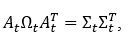 [2]
[2]where is the lower triangular matrix:
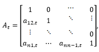
and is the diagonal matrix:
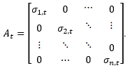
This implies that
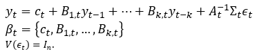 [3]
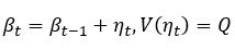
[3]The modeling strategy consists of estimating the coefficient processes in equation (3). This model has two sets of time-varying coefficients, and , and a stochastic volatility modelfor the diagonal elements, . The dynamics of the model’s time-varying parameters are specified as follows:
 [4]
[4]
 [5]
[5]
 [6]
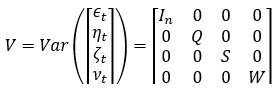
[6]where the elements of the vector are modeled as random walks as well as the free elements of the matrix . The standard deviations () are assumed to evolve as geometric random walks, which belong to the class of models known as stochastic volatility (see Blake and Mumtaz (2017)). All of the model’s innovations are assumed to be jointly normally distributed with the following assumptions on the variance covariance matrix:
 [7]
[7]where is a n-dimensional identity matrix and , and are positive definite matrices. Primiceri (2005) states these assumptions are justified, for at least two reasons: (1) the high number of parameters in the model (adding all the off-diagonal elements of would require the specification of a sensible prior that is able to prevent cases of ill-determined parameters), and (2) allowing for a completely generic correlation structure among different sources of uncertainty would preclude any structural interpretation of the innovations.
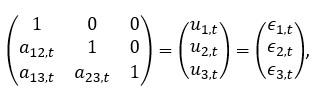
Finally, is assumed to be block diagonal, with the blocks corresponding to parameters belonging to separate equations. The intuition is that the contemporaneous relationship among variables are assumed to evolve independently in each equation. More formally, from equations (2) and (3), consider the following relationship:
 [8]
[8]In the case of a three-variable VAR, this relationship implies the following set of equations:
 [9]
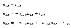
[9]which can be rearranged and translated into the following equation forms:
where and
 [10]
[10]
 [11]
[11]Therefore, the are time-varying coefficients on regressions involving the VAR residuals.
3.1.1 - Estimation procedure
Because the model includes a number of parameters that change over time, the econometric procedure for estimating the model is the Bayesian approach. In these types of models, parameters are considered latent variables so that they can be estimated with state-space models. The unobservable states correspond to the history of coefficients (, ) and the history of volatilities (). A Bayesian approach reduces uncertainty about the parameters and evaluates their posterior distribution and that of the hyperparameters ().
Gibbs sampling, a Monte Carlo with Markov Chains (MCMC) simulation method, is used for the posterior numerical evaluation of the parameters of interest. This procedure sets the prior joint distribution of the parameters function and then updates it with the data likelihood function, which generates the posterior probability function of the parameters. Because this function is analytically intractable, Gibbs sampling generates samples of the parameters from their full conditional distributions, which are smaller than their joint distribution. It is an iterative algorithm that builds sequence-dependent values of the parameters with distributions converging toward their posteriors after a number of iterations.
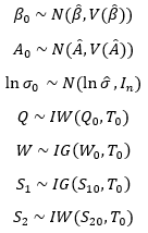
Priors. Following Blake and Mumtaz (2017), the priors for the initial states of the time- varying coefficients, simultaneous relations, and log standard errors , , and are assumed to be normally distributed. These assumptions together with the autoregressive nature of time-varying parameters imply Gaussian priors on the entire sequences of the ’s, ’s, and ’s (conditional on , , and ). The priors for the distributions of the hyperparameter is assumed to be distributed as inverse Wishart, because the parameter is inverse gamma and the blocks of are inverse gamma for and inverse Wishart for . More formally, these prior distributions have the following form:
The joint distribution of , , , and is given by

where the rectangular parenthesis is interpreted as the probability distribution and the symbol expresses proportionality.
Simulation method. A detailed explanation of the Gibbs sampling methods used to estimate the model is provided in section A.1.3 of the appendix. A summary is provided here. Following Del Negro and Primiceri (2013) and Blake and Mumtaz (2017) the Gibbs sampling algorithm is used to generate a sample from the joint posterior of (,, , and ). The algorithm is carried out in four steps, drawing (1) time-varying coefficients (), (2) simultaneous relations ( ), (3) volatilities ( ), and (4) hyperparameters (), conditional on the observed data,, and the rest of the parameters.
Conditional on and , the state-space form given by equations (3) and (4) is linear and Gaussian. Therefore, the conditional posterior of is a product of Gaussian densities and can be drawn using the Carter and Kohn (1994) algorithm. By the same logic, the posterior of conditional on and is also a product of normal distributions and can thus be drawn in the same way. Drawing instead is more complicated; this can be done using the independence Metropolis-Hastings algorithm, as presented by Blake and Mumtaz (2017). Simulating the conditional posterior of is standard because it is the product of independent inverse Wishart distributions.
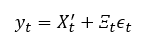
Identification. As long as an exact identification scheme —like the triangular matrix de- scribed above— for the additive shock is available, a structural vector autoregression (VAR) can be easily estimated in two steps. Consider the following structural VAR:
 [12]
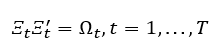
[12]where , , are matrices2 and for any , contains at least restrictions that guarantee identification. The first step consists of estimating the reduced form VAR, following the methodology illustrated in the previous sections. This first step delivers the posterior of the ’s and the ’s at every point in time. The second step is to obtain the numerical evaluation of the posterior of the ′s; it suffices to solve the system of equations given by
 [13]
[13]for every draw of . If the identification is based on a triangular scheme, the solution to (12) is given simply by , the same as in equation (3).
Sign restrictions. In order to assess the time change in the degree of procyclicality of fiscal policy to terms-of-trade shocks, we identify the shock by assuming that a positive shock has the following contemporaneous macrofiscal effects:
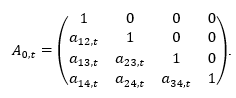
The second, third, and fourth rows of this matrix correspond to the contemporaneous response of the real exchange rate (), the primary balance (), and real GDP (), respectively, to a terms-of-trade shock. Restricting these contemporaneous responses the following way (Real Exchange Rate [RER] appreciation);, ; and , , implies that a contemporaneous shock leads to (1) a contemporaneous RER appreciation, (2) a fall in (e.g., an increase in primary expenditures that is not proportional to the increase in revenues) and (3) a contemporaneous increase in (e.g., as higher oil income increases domestic demand, both public and private).
To answer the question of whether there is an increase in fiscal procyclicality over time, one has to compare the dynamic behavior of the contemporaneous fiscal response to oil price impulses. Accordingly, we compare the contemporaneous response of the primary balance, , over time. If (where ) during the period considered, fiscal procyclicality deteriorates. Conversely, if, fiscal procyclicality improves.
The same criterion is applied to assess the direct multiplier effect of terms-of-trade shocks on the economy as well as their indirect multiplier effect (through fiscal policy). If and , then terms-of-trade shocks have a higher multiplier effect on the economy, whereas if and the opposite occurs: the multiplier effect of terms-of-trade shocks on the economy is lower. The procedure to drawing matrix is detailed in Appendix B.
4 - Data and stylized facts
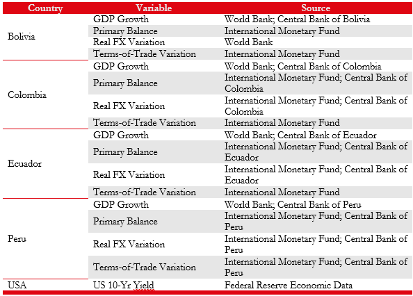
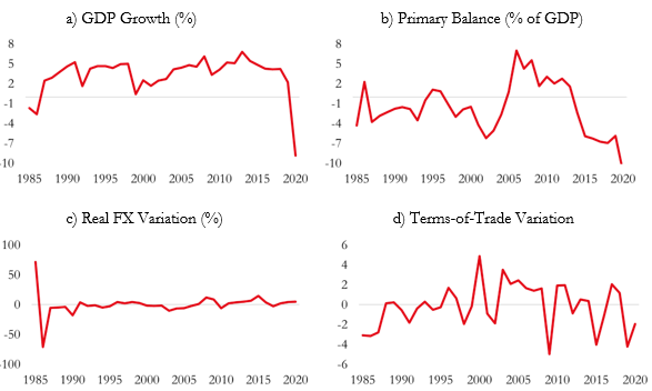
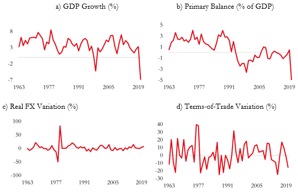
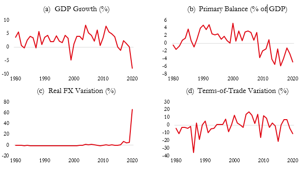
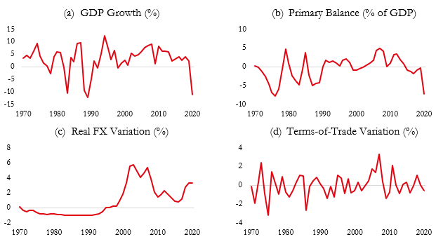
This section provides a general overview of macroeconomic performance and the fiscal framework to elucidate the evolution of these countries over the past decades and an overview of the data used. This paper evaluates the impact of terms-of-trade shocks on fiscal performance and economic growth in the countries of the Andean region. In addition to a variable that captures the terms-of-trade dynamics, the VAR model for each country includes the following variables: Economic Growth, Primary Balance (Fiscal Measure), and Real Exchange Rate (Monetary Measure). This framework enables the capture of the main transmission channels, which is necessary to explain the impacts generated by terms-of-trade shocks. The data’s periodicity is annual and the length of the periodicity depends on the availability of data for each country. Table 1 outlines the variables and sources by country, while Figures 1, 2, 3, and 4 illustrate the evolution of the series over their respective periods.
Each country in the Andean region has experienced significant economic crises that have shaped their economic and fiscal policies. Bolivia experienced a debt crisis and hyperinflation from 1977 to 1986, followed by a financial crisis from 1998 to 2002. Despite these challenges, Bolivia maintained consistent GDP growth from the late 1980s until 2019, with only brief periods of negative growth, notably in the mid-1980s and during the COVID-19 pandemic in 2020 (Kehoe et al., 2022). Colombia faced high inflation and fiscal deficits between 1971 and 1990, culminating in a severe economic recession in 1999. The COVID-19 pandemic also caused a significant GDP contraction in 2020. Throughout these periods, Colombia’s fiscal and monetary policies evolved, with significant reforms introduced following the 1991 constitution (Perez-Reyna & Osorio-Rodriguez, 2021). Ecuador’s economic history is marked by the discovery of oil reserves in the late 1960s and dollarization in 2000. The country experienced a severe economic crisis in 1999 due to political instability and central banking reforms, with GDP growth rebounding post-dollarization and another significant decline during the COVID-19 pandemic (Cueva & Díaz, 2021). Peru faced accelerating inflation and hyperinflation during the 1970s and 1980s, followed by a stabilization program in the early 1990s that led to more sustainable economic growth. Despite this, Peru experienced periods of negative growth, particularly at the end of the commodities supercycle and during the COVID-19 pandemic (Martinelli & Vega, 2021).
The fiscal performance of these countries has been influenced by their responses to eco- nomic crises and their implementation of fiscal rules. Each country has adopted various measures to improve fiscal stability and manage public finances more effectively. Bolivia has not implemented a formal fiscal rule for executing the public budget, which has led to fluctuations in the primary balance, particularly during economic downturns such as the COVID-19 pandemic (Kehoe et al., 2022). Colombia introduced significant fiscal reforms with the 1991 constitution, including the independence of the central bank and new fiscal rules in 2011. These rules target structural balance and allow for countercyclical spending, contributing to fiscal stability despite economic shocks (Perez-Reyna & Osorio-Rodriguez, 2021; Barreix & Corrales, 2019). Ecuador has implemented various fiscal rules, including spending, balance, and debt rules, to improve fiscal performance. The 2018 fiscal responsibility framework limits spending growth and restricts the deficit, aiming to maintain the debt burden below 40 percent of GDP in the medium to long term (Arenas de Mesa & Mosqueira, 2021; Barreix & Corrales, 2019). Peru’s fiscal institutional framework has undergone significant changes since the early 1990s. The Law of Fiscal Prudence and Transparency, enacted in 1999, and subsequent fiscal rules have contributed to improved fiscal performance. The 2013 Law for the Strengthening of Fiscal Responsibility and Transparency established new fiscal rules and created an independent fiscal council and a Fiscal Stabilization Fund (Martinelli & Vega, 2021; Arenas de Mesa & Mosqueira, 2021; Barreix & Corrales, 2019). The Andean Region countries have faced significant economic challenges, prompting re- forms in fiscal policies and institutional frameworks to enhance fiscal stability and economic growth. While each country has unique experiences, common themes include responses to economic crises, implementation of fiscal rules, and efforts to improve fiscal responsibility and transparency. These efforts to address fiscal imbalances and enhance economic resilience illustrate the importance of robust fiscal institutions and policies in mitigating the impacts of external shocks and promoting long-term growth.
5 - Results
5.1 - Bolivia
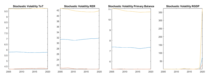
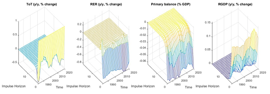
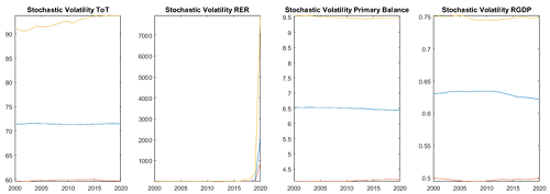
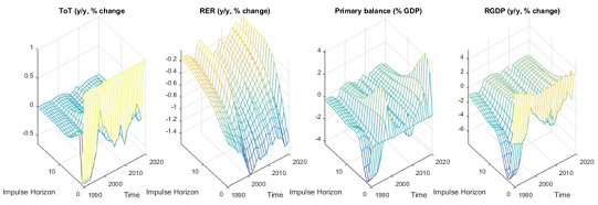
Figure 5 depicts the stochastic volatility of structural shocks for the four variables considered in the TV-SVAR, including the confidence interval computed for the shock’s 16th and 84th percentiles of the standard deviation. In the case of Bolivia, the shocks studied do not show high variability in the period considered, a behavior that contrasts with the results obtained for the other countries in the region. This result may reflect the lower development of public economic institutions in Bolivia in comparison with such institutions in the other countries in the Andean region and a lower degree of integration with the global economy. It should be noted that the limited historical availability of information only allows us to estimate the behavior of these shocks from 2005 onward.
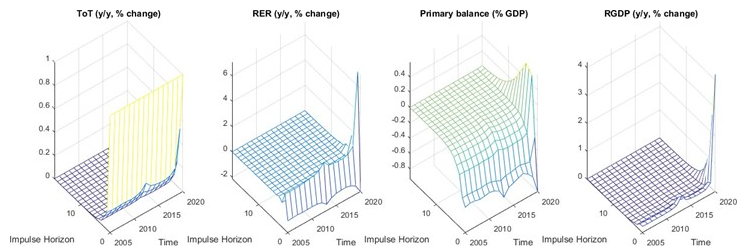
Figure 6 shows the impulse response functions of the variables considered in relation to terms-of-trade shocks over time (identified by sign restrictions). The years considered in the study are shown along the x-axis, the magnitude of the shock. along the y-axis, and the behavior of the impulse response function each year (for the periods 1 to 15) along the z-axis. In line with Bolivia’s commodity-exporting position, positive terms-of-trade shocks are associated with an appreciation of the country’s exchange rate in the initial period, followed by a depreciation, the effect of which dissolves over time. However, this effect is not pronounced, due to the country’s fixed exchange rate system. Regarding the fiscal effect of the terms-of-trade, the results show a procyclical behavior. Thus, positive shocks are associated with a more significant increase in public spending than in income during the period considered. This effect tends to be greater around 2013. Along these lines, output dynamics reflect the positive effect of terms-of-trade shocks on Bolivian economic growth. This effect may be associated with higher public spending and its economic multiplier effect.
5.2 - Colombia
In the case of Colombia, the results reveal different volatility levels among the variables’ shocks over time. Concerning the terms-of-trade, the results show a sustained increase in the volatility of the shocks during the period 2008—2014. This behavior reflect a greater dependence on oil in the country’s export basket and therefore reflect greater sensitivity of the terms-of-trade to the international price of oil and the so-called “commodity super cycle”. The results show a peak of uncertainty in 2014 associated with the fall in the international price of oil.
The volatility of shocks related to the RER showed a downward trend during the period considered, although with some volatility peaks before the year 2000. This behavior can be attributed to the country’s institutional development in economic terms, which contributed to a gradual reduction in inflation and better monetary policy management. Thus, although the country’s exchange rate continued to act as an automatic stabilizer of external shocks, the improved institutional development in monetary terms made it possible to reduce the relative size of these shocks, making for a “stable” fluctuation of the exchange rate.
On the other hand, in terms of the primary balance shocks present relatively constant volatility during the period of analysis. However, there are peaks of uncertainty related to periods of global economic recession (2000, 2008, and 2020).
Finally, in terms of economic growth, the shocks show a slight negative trend, which is in line with the relative macroeconomic stability of the country and the proper functioning of the economic institutions implemented over the last few years.
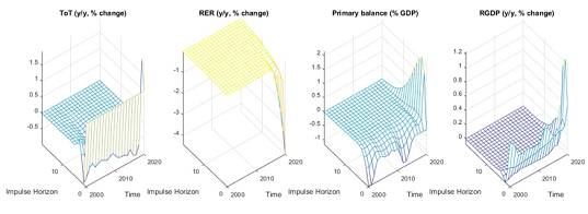
The impulse response functions reveal important changes in the magnitude of the shocks over time for the different variables. In terms of the behavior of the RER, terms-of-trade shocks had an initial appreciation effect on the rate (-0.6 p.p. to -0.8 p.p.), followed by a slight depreciation effect in subsequent periods. This behavior is present during all the years considered. The impact on initial appreciation became much stronger during the 2008—2015 period, which coincides with one of the periods of the country’s most significant oil and coal production and high international prices of these commodities. As a result of the end of the commodity super cycle, the impact of terms-of-trade shocks on the RER returned to levels similar to those evidenced before the mining-energy boom. This high exchange rate sensitivity to external shocks reflects the country’s inflation target regime, which allows the exchange rate to act as an automatic stabilizer in the face of external shocks.
Concerning the primary balance, terms-of-trade shocks show a procyclical behavior throughout the years. In this sense, improvements in the terms-of-trade generate a deterioration in the country’s fiscal position, which may be associated with a much more pronounced in- crease in spending than in income generated by better terms-of-trade. However, since 2010 there was a slight reduction in fiscal procyclicality, which coincided with a period of greater exploitation of natural resources in the country. This improvement could be related to the establishment of a fiscal rule and the development of fiscal institutions in the country in order to make good use of resources derived from extractive industries. Despite this progress, there was a tendency toward greater procyclicality in the last few years of the period under study.
Finally, terms-of-trade shocks show a positive effect on economic growth. The most significant impact of these shocks (0.15 p.p) was felt from 2010 to 2015, coinciding with the commodity cycle and the country’s mining-energy boom.
5.3 - Ecuador
In the case of Ecuador, the behavior related to the volatility of the different shocks remained relatively constant over time (Figure 9). In terms of impulse response functions, except for the RER behavior, the different variables show a changing reaction over time. The dollarization of the economy explains the low effect of terms-of-trade shocks on the RER. However, due to the crisis generated by the pandemic and the local and foreign price differentials, the RER showed a differential impact during 2020. Regarding fiscal variables, positive terms-of-trade shocks generate a higher deficit, in line with a procyclical behavior of fiscal policy. The procyclicality of spending presented a greater magnitude between 2010 and 2013, coinciding with the commodity super cycle. In terms of economic growth, due to the country’s commodity-exporting position favorable terms-of-trade shocks are positively related to higher economic growth, especially in the 2000—2003 and 2010—2013 periods.
5.4 - Peru
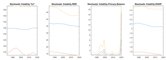
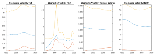
In Peru, the behavior of the volatility of shocks shows high variability, especially in the case of terms-of-trade and RER shocks (Figure 11). The terms-of-trade volatility shows a peak of uncertainty in the period corresponding to the 2008 global financial crisis and the sharp fall in international copper prices that occurred. From this point on, the magnitude of the shocks shows a considerable decrease with some minor peaks in 2014, coinciding with the end of the commodity super cycle. When examining the behavior of the RER, the shocks present high volatility with a significant peak of uncertainty around the year 2003, which coincides with a period of appreciation of the local currency. Finally, the volatility of fiscal and economic growth shocks shows less variation, although with a marked negative trend, mainly in the case of GDP performance. This result may be associated with more economic stability in Peru due to the strengthening of its fiscal institutions in recent years.
When examining the behavior of the terms-of-trade shocks in the variables considered, we observe in all cases a response that varies significantly according to the years considered (Figure 11). In the case of the response in the RER, the exchange rate appreciation effect that occurs after a positive terms-of-trade shock is of a greater magnitude in the period close to the year 2000 (-2.0 p.p.). A trend of greater sensitivity of the RER is also observed as of 2015, although at much lower levels (-1.5 p.p.) than those recorded in 2000. This result may be related to changes in the Peruvian monetary authorities’ exchange rate intervention policy to maintain price stability per the established policy objectives.
Regarding the primary balance, terms-of-trade shocks show a differentiated effect depending on the years considered. From 1990 to 1997, trade shocks were associated with a negative response of the primary balance (higher deficit). However, from 2000 on (except for a few years, notably 2005 and 2010) terms-of-trade shocks resulted in an improvement of the primary balance. This may be because of improved fiscal institutions that allowed the country to implement a countercyclical fiscal policy. In terms of GDP performance, the response of economic growth to terms-of-trade shocks was similar to that of the primary balance. From 2000 on, positive terms-of-trade shocks were associated with positive economic activity.
5.5 - Responses to a Terms-of-Trade Shock for Selected Periods
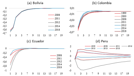
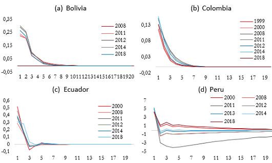
Figures 13 and 14 show the responses of the primary balance and of economic growth, respectively, to terms-of-trade shocks at different points in time. The periods of interest in which the impulse response functions (IRFs) are calculated respond both to periods of global shocks (international financial crisis, commodity super cycle) and periods in which significant changes occurred in the countries’ fiscal institutions (fiscal rules going into effect or new institutional arrangements).
Figure 13 reveals that, with the exception of Peru, the countries of the Andean region show an increase in their deficit as a consequence of a positive terms-of-trade shock. In other words, the fiscal balance reflects a procyclical behavior in public finances. Bolivia is the country that shows the greatest sensitivity to the shocks considered, with 2014 being the year with the most pronounced response in its primary balance (-0.66 p.p.) and 2008 the year with the lowest response (-0.6). For this country, no significant heterogeneity is observed between the different time periods considered. In the case of Colombia, the country’s primary balance shows a much smaller reaction than that of the other countries considered, with the year 2000 seeing the greatest impact (-0.06 p.p.), which makes sense given the 1999 Colombian economic crisis. The 2014 shock is associated with a lower impact (-0.05). In Ecuador, the response to shocks varies over the period of study. Thus, the largest (negative) impact on the primary balance was felt in 2012, when there was a significant increase in the international price of oil. As mentioned above, this behavior responds to a procyclical policy by the economic authorities. In contrast, in 2018 the impact on the deficit was much lower (- 0.27), a result that may be correlated with the development of better fiscal institutions in Ecuador during the last few years of the period under study. Finally, Peru is the country in the region that shows the most variable responses to terms-of-trade shocks. The largest shock for Peru occurred in 2011, with a deficit shock of -3.0 p.p. that also showed high persistence. This strong shock may capture the decline in copper prices as a consequence of the international financial crisis and the other effects of the global economic recession on the local economy. On the other hand, Peru saw an improvement in its primary balance in the face of terms-of-trade shocks in 2000, 2015, and 2018. This result may be associated with the strengthening of Peruvian economic institutions in recent years. In this sense, our results demonstrate significant differences between the effects that terms-of-trade shocks generate in the countries of the region and the heterogeneity of each country’s response during the period of study.
In terms of the impact on growth of terms-of-trade shocks, Figure 14 presents behaviors in line with the fiscal policies carried out by the countries. Positive terms-of-trade shocks generate higher economic growth in all countries, with the exception of some years in the case of Peru (2011, 2012, 2014). This behavior correlates with the higher public spending and infrastructure investment programs undertaken by the countries in the region made possible by mining and energy tax revenues and their multiplier effect on the economy. Ecuador and Peru show the greatest impact on economic growth derived from positive terms-of-trade shocks, while Colombia shows the least sensitivity.
6 - Concluding Remarks
This paper examines the impact of terms-of-trade shocks on fiscal performance and eco- nomic growth in the Andean region, employing a Time-Varying Structural Vector Autoregression (TV-SVAR) model, following the methodology proposed by Primiceri (2005), to capture the dynamic responses of key macroeconomic variables over time. The results re- veal significant heterogeneity across Bolivia, Colombia, Ecuador, and Peru, both within and between countries, in terms of the volatility and transmission of external shocks, reflecting differences in institutional quality and fiscal policy frameworks.
The study shows that, within countries, terms-of-trade shocks exhibit significant time- varying behavior, with more pronounced effects during the commodity super cycle period. Positive terms-of-trade shocks, such as increases in commodity prices, are generally associated with higher public spending and economic growth, indicating procyclical fiscal behavior. However, countercyclical responses are observed in certain years, particularly in Peru, where more robust fiscal frameworks have been developed. Bolivia and Ecuador exhibit the most pronounced procyclical fiscal responses, with government spending sharply increasing during periods of favorable external conditions. This behavior has led to substantial fiscal imbalances during downturns, underscoring the need for stronger fiscal institutions in these countries.
In contrast, Colombia and Peru have demonstrated greater resilience to external shocks due to the implementation of fiscal rules and stabilization mechanisms that have enabled them to moderate the impact of terms-of-trade volatility on public finances, resulting in more stable macroeconomic outcomes. The analysis emphasizes the importance of fiscal institutions, such as fiscal rules and councils, in shaping countries’ ability to manage revenue from extractive industries and implement countercyclical policies. Countries with more developed fiscal frameworks, like Colombia and Peru, are better able to smooth public spending and ensure fiscal stability, while those with weaker institutions, like Bolivia and Ecuador, remain vulnerable to the boom-bust cycles associated with commodity price fluctuations.
These findings carry significant policy implications for resource-dependent economies. Policymakers should consider the magnitude of shocks and the nonrenewable nature of resource revenues when designing fiscal policies. Public spending should align with intertemporal smoothing strategies to avoid excessive spending during boom periods, which could undermine long-term fiscal stability. Furthermore, institutional development, particularly the establishment of sound fiscal frameworks, should be a priority for countries like Bolivia and Ecuador to enhance their resilience to external shocks.
In the context of the global energy transition, the development of proper fiscal institutions becomes even more critical. The Andean countries must prepare for potential shifts in global demand for commodities and avoid significant macroeconomic instability. Economic diversification should be a key goal for the region to mitigate the risks associated with dependency on commodity exports.
Future research could explore how further institutional reforms and improvements can strengthen the resilience of these economies to external volatility. The Andean region pro- vides valuable insights into the complex interplay between external shocks, fiscal policy, and institutional capacity, offering important lessons for other commodity-exporting countries facing similar challenges.
Figures and Tables
Contribución de los/as autores/as
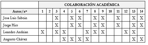
1. Administración del proyecto, 2. Adquisición de fondos, 3. Análisis formal, 4. Conceptualización, 5. Curaduría de datos, 6. Escritura - borrador original, 7. Escritura - revisión y edición, 8. Investigación, 9. Metodología, 10. Recursos, 11. Software, 12. Supervisión, 13. Validación, 14. Visualización.
References
Aguiar, M. y Amador, M. (2011). Growth in the shadow of expropriation. The Quarterly Journal of Economics, 126(2), 651-697.
Alberola, E. y Sousa, R. (2017). Assessing fiscal policy through the lens of the financial and the commodity price cycles (Working Paper 638). Bank for International Settlements.
Alesina, A., Campante, F. y Tabellini, G. (2008). Why is fiscal policy often procyclical? Journal of the European Economic Association, 6(5), 1006-1036. https://doi.org/10.1162/JEEA.2008.6.5.1006
Andrian, L. G., Hirs, J. y Valencia, O. (2023). Instituciones fiscales en los países de la Región Andina y retos derivados del proceso de descarbonización (Nota técnica 2820). Banco Interamericano de Desarrollo. https://doi.org/10.18235/0005253
Arenas de Mesa, A. y Mosqueira, E. (2021). La transformación y el fortalecimiento institucional de los Ministerios de Hacienda en América Latina: del control al uso estratégico de los recursos públicos para el desarrollo (Documentos de Proyectos LC/TS.2021/23). Comisión Económica para América Latina y el Caribe (CEPAL)/Banco Interamericano de Desarrollo (BID).
Barreix, A. D. y Corrales, L. F. (Eds.) (2019). Reglas fiscales resilientes en América Latina (Vol. 767). Inter-American Development Bank.
Barro, R. (1979). On the determination of the public debt. Journal of Political Economy, 87(5), 940-971.
Bauwens, L., Lubrano, M. y Richard, J. (1999). Bayesian inference in dynamic econometric models. Oxford University Press.
Benati, L. y Mumtaz, H. (2007). US evolving macroeconomic dynamics: A structural investigation (Working Paper Series No. 746). European Central Bank.
Bjørnland, H. C. y Thorsrud, L. A. (2019). Commodity prices and fiscal policy design: Procyclical despite a rule. Journal of Applied Econometrics, 34(2), 161-180. https://doi.org/10.1002/jae.2669
Blake, A. y Mumtaz, H. (2017). Applied Bayesian econometrics for central bankers. Centre for Central Banking Studies, Bank of England.
Caballero, R. J. y Krishnamurthy, A. (2004). Fiscal Policy and Financial Depth (Working Paper 10532). National Bureau of Economic Research.
Camacho, M. y Perez-Quiros, G. (2014). Commodity prices and the business cycle in Latin America: Living and dying by commodities? Emerging Markets Finance and Trade, 50(2), 110—137.
Carter, C. y Kohn, R. (1994). On Gibbs sampling for state space models. Biometrika, 81(3), 541-553. https://doi.org/10.2307/2337125
Casella, G. y George, E. (1992). Explaining the Gibbs Sampler. The American Statistician, 46(3), 167-174. https://doi.org/10.1080/00031305.1992.10475878
Céspedes, L. F., Parrado, E. y Velasco, A. (2014). Fiscal rules and the management of natural resource revenues: The case of Chile. Annual Review of Resource Economics, 6(1), 105-132. https://doi.org/10.1146/annurev-resource-100913-012856
Céspedes, L. F. y Velasco, A. (2012). Macroeconomic performance during commodity price booms and busts. IMF Economic Review, 60(4), 570-599.
Céspedes, L. F. y Velasco, A. (2014). Was this time different? Fiscal policy in commodity republics. Journal of Development Economics, 106(C), 92-106.
Cueva, S. y Díaz, J. P. (2021). The history of Ecuador. En T. J. Kehoe y J. P. Nicolini (Eds.), A monetary and fiscal history of Latin America, 1960–2017 (pp. 277—319). University of Minnesota Press.
Del Negro, M. y Primiceri, G. E. (2013). Time-varying structural vector autoregressions and monetary policy: A corrigendum (Staff Report 619). Federal Reserve Board of New York.
Erbil, N. (2011). Is fiscal policy procyclical in developing oil-producing countries? (Working Paper 171). International Monetary Fund. https://www.imf.org/en/Publications/WP/Issues/2016/12/31/Is-Fiscal-Policy-Procyclical-in-Developing-Oil-Producing-Countries-25063
Fernández, A., González, A. y Rodriguez, D. (2018). Sharing a ride on the commodities roller coaster: Common factors in business cycles of emerging economies. Journal of International Economics, 111, 99-121. https://doi.org/10.1016/j.jinteco.2017.11.008
Fernández, A., Schmitt-Grohé, S. y Uribe, M. (2020). Does the commodity super cycle matter? (Working Paper 27589). National Bureau of Economic Research. https://doi.org/10.3386/w27589
Frankel, J. A. (2010). The natural resource curse: A survey (Working Paper 15836). National Bureau of Economic Research. https://doi.org/10.3386/w15836
Frankel, J., Vegh, C. y Vuletin, G. (2013). On graduation from fiscal procyclicality. Journal of Development Economics, 100, 32-47.
Gavin, M., Hausmann, R., Perotti, R., & Talvi, E. (1996). Managing fiscal policy in Latin America and the Caribbean: Volatility, procyclicality and limited creditworthiness. Inter-American Development Bank. http://dx.doi.org/10.18235/0011562
Gavin, M. y Perotti, R. (1997). Fiscal policy in Latin America. En B. S. Bernanke y J. J. Rotemberg (Eds.), NBER Macroeconomics Annual 1997 (vol.12, pp. 11—70). MIT Press.
Harberger, A. C. (1950). Currency depreciation, income, and the balance of trade. Journal of Political Economy, 58(1), 47-60. https://doi.org/10.1086/256897
Ilzetzki, E. (2011). Rent-seeking distortions and fiscal procyclicality. Journal of Development Economics, 96(1), 30-46. https://doi.org/10.1016/j.jdeveco.2010.07.006
Ilzetzki, E. y Vegh, C. (2008). Procyclical fiscal policy in developing countries: Truth or fiction? (Working Paper 14191). National Bureau of Economic Research. https://doi.org/10.3386/w14191
Izquierdo, A., Romero, R. y Talvi, E. (2008). Booms and busts in Latin America: The role of external factors (Working Paper 631). Inter-American Development Bank. http://dx.doi.org/10.18235/0010885
Jacquier, E., Polson, N. y Rossi, P. (2004). Bayesian analysis of stochastic volatility models. Journal of Business and Economic Statistics, 12(4), 371-418. https://doi.org/10.1080/07350015.1994.10524553
Jemio, L. C. (2006). Volatilidad externa y el sistema financiero en Bolivia. Informe de consultoría elaborado para la Corporación Andina de Fomento (CAF).
Kalmanovitz, S. (2017). Breve historia económica de Colombia. Biblioteca Nacional de Colombia. Ministerio de Cultura.
Kaminsky, G. L., Reinhart, C. M. y Végh, C. A. (2004). When it rains, it pours: Procyclical capital flows and macroeconomic policies (NBER Working Paper No. 10780). National Bureau of Economic Research.
Kehoe, T. J. y Nicolini, J. P. (Eds.). (2022). A monetary and fiscal history of Latin America, 1960—2017. University of Minnesota Press.
Kehoe, T. J., Machicado, C. G. y Peres-Cajías, J. (2022). The history of Bolivia. En T. J. Kehoe y J. P. Nicolini (Eds.), A monetary and fiscal history of Latin America, 1960—2017 (pp. 83—129). University of Minnesota Press.
Kim, C. y Nelson, C. (1999). State-space models with regime switching. MIT Press.
Kose, M. (2002). Explaining business cycles in small open economies: “How much do world prices matter?” Journal of International Economics, 56(2), 299-327.
Lane, P. y Tornell, A. (1996). Power, growth and the voracity effect. Journal of Economic Growth, 1(2), 213-241. https://doi.org/10.1007/BF00138863
Laursen, S. y Metzler, L. A. (1950). Flexible exchange rates and the theory of employment. The Review of Economics and Statistics, 281-299.
Levy, A., Ricci, L. A. y Werner, A. M. (2020). The sources of fiscal fluctuations (Working Paper 2020/220). International Monetary Fund.
Mankiw, N. G. y Romer, D. (1991). New Keynesian Economics (2 vols.). MIT Press.
Martinelli, C. y Vega, M. (2021). The history of Peru. En T. J. Kehoe y J. P. Nicolini (Eds.), A monetary and fiscal history of Latin America, 1960–2017 (pp. 401—448). University of Minnesota Press.
Medina, L. (2016). The effects of commodity price shocks on fiscal aggregates in Latin America. IMF Economic Review, 64(3), 502-525. https://doi.org/10.1057/imfer.2016.14
Melo-Becerra, L. A., Parrado-Galvis, L. M., Ramos-Forero, J. E. y Zarate-Solano, H. M. (2020). Efectos de los auges y la crisis del petróleo en la economía colombiana: un enfoque autorregresivo vectorial variable en el tiempo. Revista de Economía del Rosario, 23(1), 31-63. https://doi.org/10.12804/revistas.urosario.edu.co/economia/a.8631
Mendoza, E. G. (1995). The terms-of-trade, the real exchange rate, and economic fluctuations. International Economic Review, 36(1), 101-137. https://doi.org/10.2307/2527429
Nakajima, J., Kasuya, M. y Watanabe, T. (2011). Bayesian analysis of time-varying parameter vector autoregressive model for the Japanese economy and monetary policy. Journal of the Japanese and International Economies, 25(3), 225-245. https://doi.org/10.1016/j.jjie.2011.07.004
Ostry, J. D. y Reinhart, C. M. (1992). Private saving and terms-of-trade shocks: Evidence from developing countries. IMF Staff Papers, 39(3), 495-517.
Perez-Reyna, D. y Osorio-Rodriguez, D. (2021). The history of Colombia. En T. J. Kehoe y J. P. Nicolini (Eds.), A monetary and fiscal history of Latin America, 1960–2017 (pp. 243—274). University of Minnesota Press.
Petrova, I., Papaioannou, M. G. y Bellas, D. (2010). Determinants of emerging market sovereign bond spreads: Fundamentals vs financial stress (Working Paper No. 2010/281). International Monetary Fund.
Primiceri, G. E. (2005). Time varying structural vector autoregressions and monetary policy. The Review of Economic Studies, 72(3), 821-852. https://doi.org/10.1111/j.1467-937X.2005.00353.x
Ramirez, J., Waggoner, D. y Zha, T. (2010). Structural vector autoregressions: Theory of identification and algorithms for inference. Review of Economic Studies, 77(2), 665-696.
Riascos, A. y Vegh, C. A. (2003). Procyclical government spending in developing countries: The role of capital market imperfections [Mimeo]. UCLA and Banco de la República, Colombia.
Stein, E., Talvi, E. y Gristani, A. (1999). Institutional arrangements and fiscal performance: The Latin American experience. En J.M. Poterba y J. von Hagen (Eds.), Fiscal institutions and fiscal performance (pp. 103-134). University of Chicago Press.
Tornell, A. y Lane, P. R. (1999). The voracity effect. American Economic Review, 89(1), 22-46. https://doi.org/10.1257/aer.89.1.22
Tornell, A. y Velasco, A. (1992). The tragedy of the commons and economic growth: Why does capital flow from poor to rich countries? Journal of Political Economy, 100(6), 1208-1231. https://doi.org/10.1086/261858
Villafuerte, M. y Lopez-Murphy, P. (2009). Fiscal policy in oil producing countries during the recent oil price cycle (Working Paper WP/10/28). International Monetary Fund.
Zeev, N. B., Pappa, E., & Vicondoa, A. (2017). Emerging economies business cycles: The role of commodity terms-of-trade news. Journal of International Economics, 108, 368—376.
Zellner, A. (1971). An introduction to Bayesian inference in econometrics. Wiley.
A. Sampling algorithms for estimation of model parameters
A.1 Drawing coefficient states
A.1.1 A standard state-space representation
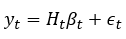
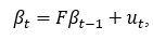
Equations (3) and (4) have, respectively, the state-space form of equations (14), the “observation” equation, and (15), the “transition” equation, below:
 [14]
[14]
 [15]
[15]where
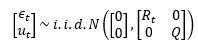
In the observation equation the unknown parameters consist of the elements of H not fixed or given as data and the nonzero elements of the covariance matrix R. In the transition equation, the parameters to be estimated are the nonzero and free elements of F, Q, and the state variable, .
A.1.2 Bayesian econometrics: The general procedure
A Bayesian approach to estimating this model is based on three basic steps.
Step 1. The researcher forms a prior belief of the distribution of the parameters to be estimated , where is a generic joint density function of the parameters.
Step 2. The researcher collects data on the observed variables () and constructs the likelihood function of the model parameters contained in the data .
Step 3. The researcher updates the prior belief on the model parameters (step 1) based on the information contained in the data (step 2). Put another away, the researcher combines the prior distribution and the likelihood function to obtain the joint posterior distribution .
Defined by Bayes’ theorem, is a product of the likelihood and the joint prior . More formally,

here indicates proportionality.
To proceed further in terms of inference, the researcher has to “isolate” the component of the posterior relevant to the parameter of interest. For example, to conduct inference about β, the researcher has to derive the marginal posterior distribution for β from the joint posterior distribution of the parameters. Similarly, inference on Q is based on the marginal posterior distribution for Q. However, derivation of the marginal posterior distribution (from a joint posterior distribution) requires analytical integration, a procedure that may prove difficult in complex models such as the one used here. It was the development of simulation methods such as Gibbs sampling that greatly simplified this integration.
A.1.3 Bayesian econometrics: The general procedure
Gibbs sampling is a numerical method that use draws from conditional distributions to approximate joint and marginal distributions. From Blake and Mumtaz (2017), a general description of Gibbs sampling is the following:
Suppose we have a joint distribution of variables
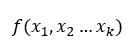
This may, for example, be a joint posterior distribution.
We are interested in obtaining the marginal distributions
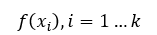
Assume that the form of the conditional distributions , is known. A Gibbs sampling algorithm with the following steps can be used to approximate the marginal distributions:
(1) Set starting values for

Where the superscript 0 denotes the starting values.
(2) Sample from the distribution of conditional on current values of
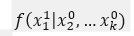
(3) Sample from the distribution of conditional on current values of
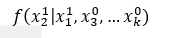
(4) Sample from the distribution of conditional on current values of
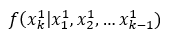
to complete 1 iteration of the Gibbs sampling algorithm.
As the number of Gibbs iterations increases to infinity, the samples or draws from the conditional distributions converge to the joint and marginal distributions of at an exponential rate (for a proof of convergence see Casella and George (1992)). More concretely, by repeating the Gibbs sampling algorithm M times (i.e., a large enough number to achieve convergence) and saving the last H draws of , we obtain H values for . A histogram for is an approximation for the marginal density of . One crucial thing to note is that the implementation of the Gibbs sampling algorithm requires the researcher to know or assume the form of the conditional distributions .
A.1.4 Gibbs sampling in state-space models
Going back to the state-space model of equations (14) and (15) above, a Gibbs sampling algorithm for this problem can be constructed by assuming that the state variable, is known and observed. This observation implies the following general Gibbs algorithm:
Step 1. Conditional on , sample H and R from their posterior distributions.
Step 2. Conditional on , sample F and Q from their posterior distributions.
Step 3. Conditional on the parameters of the state-space (F, H, Q, R), sample from its conditional posterior distribution.
Step 4. Repeat steps 1 to 3 until convergence is achieved.
As shown by Carter and Kohn (1994), the conditional posterior distribution, where is the time series vector of (the same applies to ), can be factored into the following conditional distributions.
 [16]
[16]Note that the right-hand side splits into the product of (1) the marginal distribution of the state-space variable at time T and (2) the distribution of the vector conditioned on (i.e., its conditional posterior). As shown in Kim & Nelson (1999), considering the fact that follows a first-order autoregressive or Markov process, equation (16) can be rewritten as

where, given that and u_t are normally distributed:

Then, to draw ’s from this distribution we need to calculate its mean, , and variance, , using the Kalman filter:


Starting from an initial value, that is, a prior of state and variance of the state , a standard Kalman filter consists of the following equations, which are evaluated recursively through time:
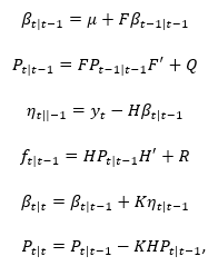
Where is the “Kalman gain” (i.e., the weight attached to the prediction error). Running these equations from delivers and at the end of the recursion, which are known as the “updating” equations as they update the initial estimates and using information contained in the prediction error, .
Finally, the draw of and the output of the filter are now used for the first step of the backward recursion (which provides and used to make a draw of . This process can be thought as updating (the Kalman filter estimate of the state variable) for information contained in . This backward recursion continues until time zero. As shown in Blake and Mumtaz (2017, p. 74), for a given time t, the updating formulas of the backward recursion are

The above formulas constitute the Carter and Kohn algorithm.
A.1.5 Drawing βt’s
Equations (14) and (15) can be rewritten as the following state-space forms:
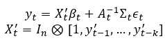 [17]
[17]
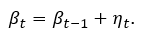 [18]
[18]The observation equation (17) is linear and has Gaussian innovations with known variance. Following the procedure described in Section A.1.4, the conditional posterior distribution can be factored as

where

Then, to draw ’s from this distribution we need to calculate its state mean, , and state variance, :
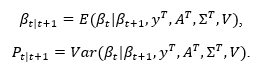
The vector of 's can be easily drawn because it can be computed using the forward (Kalman filter) and the backward (Carter and Kohn algorithm) recursions presented in Section A.1.4.
The starting values of the Kalman filter, that is, the prior of the state and variance of the state are the following:
Priors for ’s. The first observations of the sample (the 20-year period 1962—1981) are used to estimate a standard fixed-coefficient VAR via ordinary least squares (OLS) such that with a coefficient covariance matrix given by , where , and the subscript denotes the fact that this is the training sample.
The last recursion of the Kalman filter provides , and which are the mean variance of the posterior distribution of . After drawing a value from this distribution, the draw is used in the backward recursion to obtain and from period to , that is, to obtain conditional on .
A.1.6 Drawing aij,t 's
From equations (8) to (11), state-space formulations for the ’s can be derived. Specifically, the state-space formulation for is
 [19]
[19]
 [20]
[20]and the state-space formulation for and is
 [21]
[21]
 [22]
[22]Because S is block diagonal, the Kalman filter and Carter and Kohn algorithm can be applied equation by equation. The priors of the are the following:
Priors for s. Let and ley denote the inverse of the matrix with the diagonal normalized to 1 . The initial values for (i.e., the initial state ) are the nonzero of A_0 with the variance of the initial state set equal to , following Benati & Mumtaz (2007).
Note that without the block diagonality of it would not be feasible to apply the Kalman filter and Carter and Kohn algorithm equation by equation and draw separately every block of ’s. However, while the block-diagonal assumption of simplifies the analysis, it is not essential and Primiceri (2005) provides a procedure to deal with an unrestricted .
A.2 Drawing volatilities
A.2.1 The Metropolis Hasting algorithm
In this section, following Blake and Mumtaz (2017), we briefly describe the Metropolis Hastings (MH) algorithm in a general setting. Suppose that we are interested in drawing samples from the following distribution:

where is a vector that represents a set of parameters and is referred as the “target density.” can be thought of a posterior distribution where the Gibbs sampler is not operation, because the conditional distributions of different blocks of the parameters are unknown. However, if provided with a value of it is possible to evaluate the density of , that is, . If this is the case, the MH algorithm can be used to sample from following the steps described below:
Step 1. Specify a candidate density where indexes the draw of the parameters . One must be able to draw samples from this density.
Step 2. Draw a candidate value of the parameters from the candidate density .
Step 3. Compute the probability of accepting (denoted by ) using the expression
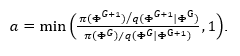
The numerator of this expression is the target density evaluated at the new draw of the parameters divided by the candidate density evaluated at the new draw of the parameters . The denominator is the same expression evaluated at the previous draw of the parameters
Step 4. If the acceptance probability α is large enough, retain the new draw , otherwise retain the old draw . We decide if α is large enough by drawing a number u from the standard uniform distribution. If , accept ; otherwise keep 3.
Step 5. Repeat steps 2 to 4 times and base inference on the last draws. Provided convergence exists, the empirical distribution using the last draws is an approximation to target density.
A.2.2 A simple stochastic volatility model using the MH algorithm
Consider the simple stochastic volatility model
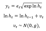
where is time-varying variance. This is a state-space model where the observation equation is nonlinear in terms of the state variable and therefore the Carter and Kohn algorithm does not apply. Jacquier et al. (2004) suggest applying an independence MH algorithm at each t to sample from the conditional distribution of which is given by where the subscript denotes all other dates than .
Because the transition equation is a random walk, the knowledge of and contains all the relevant information about . This way, the conditional distribution of can be simplified as

To sample from a date-by-date application of the independence MH algorithm could be performed following steps 2 to 4 as described in Section A.2.1. However, this procedure does not apply for the first and last observations. Therefore, the general algorithm is modified as follows (Blake & Mumtaz, 2017, p. 158): Jacquier et al. (2004) show that this density has the following form:

that is, this density is the product of a normal density and a log normal density, with
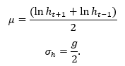
Step 1. Generate a starting value for as and set the prior, (e.g, could be the log of the OLS estimate of the variance of and could be set to a big number to reflect the uncertainty in this initial guess). Set an inverse-gamma prior for g (i.e.,). Set a starting value for g.
Step 2. The drawing of proceeds in three steps:
2a. for t=0 , sample the initial value of denoted by from the log normal density
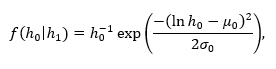
where the mean and .
2b. For each date to draw a new value for h_t from the candidate density (call the draw )
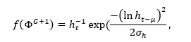
Where and . Compute the acceptance probability
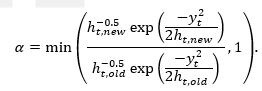
Draw . If , set . Otherwise retain the old draw.
2c. For the last time period compute and and draw from the candidate density
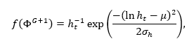
Compute the acceptance probability
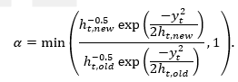
Draw . If , set . Otherwise retain the old draw.
Step 3. Given a draw for , compute the residuals of the transition equation . Draw g from the inverse-gamma distribution with scale parameter and degrees of freedom .
Step 4. Repeat steps 2 and 3 M times. The last L draws of and provide an approximation to the marginal posterior distributions.
A.2.3 Drawing (σi,t)’s
Equations (3) and (6) can be rewritten into the following state-space forms:
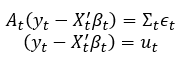 [23]
[23]
 [24]
[24]where is time-varying variance. This is a state-space model where the observation equation is nonlinear in the state variable σ and therefore can be estimated by the MH algorithm explained above after linearization. Note that because is contemporaneously uncorrelated, the draws from the MH algorithm can be done separately for each .
Priors for . A starting value for is obtained from . The prior for can be set equal of the ith diagonal element of and to a large number, 10 in this case, following Blake and Mumtaz (2017).
A.3 Drawing hyperparameters
Conditional on , , , and , it is easy to draw posteriors using Gibbs sampling for , the block of , and , because all of these posteriors are observable. We discuss the priors we used to estimate these conditional distributions below.
A.3.1 Priors
The first observations (the 20-year period between 1962 and 1981) are used to calibrate the prior distributions.
Prior for . The (conjugate) prior for is inverse-Wishart4 , where is the scale matrix and are the degrees of freedom. This prior is key, because it shapes the amount of time variation allowed for in the VAR model, that is, a large value for the scale matrix would imply more fluctuation in .
The scale matrix is set equal to , where τ is a scaling factor chosen by the researcher. Some studies set , i.e., a small number, to reflect the fact that the training sample is typically short and the resulting estimates of maybe imprecise. Note that one can control the a priori amount of time variation in the model by varying .
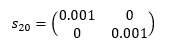
Priors for and . The prior for is inverse-gamma5 and the prior for is inverse Wishart . We follow Benati & Mumtaz (2007) who set and .
Priors for . An inverse-gamma prior for is set with scale parameter and degrees of freedom .
A.3.2 Posteriors
Posterior for . The hyperparameter has an inverse-Wishart conditional posterior distribution . Posteriors for and . The hyperparameter has an inverse-gamma posterior conditional distribution . Posterior for Q. The hyperparameter Q has an inverse-Wishart conditional posterior distribution
Posteriors for and . The hyperparameter has an inverse-gamma posterior conditional distribution .
The hyperparameter has an inverse-Whishart conditional posterior .
Posterior for . The hyperparameters in have an inverse-gamma conditional posterior distribution .
A.4 Summary of the sampling chain
Step 1. Set priors and initial values of , , , , the block , and :
1a. Set prior for : and starting values of the Kalman filter: and .
1b. Set prior for :, a prior for :, and starting values of .
1c. Set a starting value for and a prior for : .
Step 2. Conditional on , , and , draw using the Carter and Kohn algorithm.
Step 3. Conditional on the draw of , sample from .
Step 4. Conditional on , , and and , draw using the Carter and Kohn algorithm.
Step 5. Conditional on the draw of estimate residuals , , , and sample from and from . .
Step 6. Using the draw of from Step 4, calculate and draw using the MH algorithm.
Step 7: Conditional on a draw for , draw from .
Step 8: Repeat steps 2 to 7 times. The last draws give an approximation to the marginal posterior distribution of the model parameters.
B Algorithm for sign restrictions
Once past the burn-in stage –the process of dropping Gibbs draws– and marginal posterior distributions of all the model’s parameters are obtained, following Ramirez (2010), the steps presented below are used to calculate the required matrix with sign restrictions:
Step 1. Draw a matrix from the standard normal distribution.
Step 2. Calculate the matrix from the decomposition of . Note that is orthonormal i.e., .
Step 3. Calculate the Cholesky decomposition of the current draw of .
Step 4. Calculate the candidate matrix as . Because , this implies that will still equal , that is, by calculating the product we alter the elements of but not the property that . The candidate matrix has the following form:
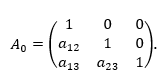
The second and third rows of this matrix corresponds to the oil price shock impact on the fiscal variable and the nonoil real GDP, respectively. We need to check if , , and . If this is the case, a contemporaneous shock in will lead to a fall in and an increase in , because the elements () correspond to the current period response of to an shock. If , , and , the algorithm stops and uses this matrix to compute a draw of impulse responses. If the restriction is not satisfied, the algorithm goes back to step 1 and tries with a new matrix.
Step 5. Repeat steps 1 to 4 for every retained Gibbs draw.
Notes
Additional information
Clasificación JEL: E62, D72, F3, H60


