1. Introduction
The quantity, quality, and timing of streamflow are crucial to sustain freshwater and estuarine ecosystems, and to certain human activities (e. g., agriculture, industry, electricity, domestic, recreation)(1). Agricultural irrigation is one of the most water-intensive activities in the world, where the farmer must have prior information of quantity and frequency of streamflows to design irrigation systems and optimize water use without undesirable environmental impacts. Flow Duration Curves (FDC) represent the relationship between the magnitude and the frequency of streamflow and provide an estimate of the percentage of time a given streamflow is equaled or exceeded over a historical period(2). FDC are obtained from long-term records of streamflow and are often used in hydropower, water-supply and irrigation projects. In practice, it is rare to have gauging stations at the project sites, for that reason hydrological simulation has become an attractive alternative to estimate FDC.
Regionalization in hydrologic models is applied to estimate streamflow at ungauged catchments because they use effective parameters that are transferred from gauged catchments to ungauged catchments(3). Narbondo and others(4) applied the regionalization of the lumped GR4J model(5) in Uruguay, where the authors used the concept of physical similarity to find relationships between model parameters and physical attributes of the catchment at the country scale. However, this type of approach can be strongly influenced by local conditions, especially in small basins(6). An elegant solution is to account for spatial variations of hydrologic processes within the catchment domain by using spatially distributed models. In addition, this technique allows implementation of novel approaches in optimization procedures through the use of soft data(7). However, these techniques are too complex to be implemented on-demand for small irrigation projects, as they require great computational coding development time and analysis.
A major drawback of hydrologic modeling is that the results are generally only used for the researchers who developed the model, because the format of the model outputs are complex and difficult to share. In recent years, the open-source programming language R(8) has emerged as a solution as it has extensive benefits, such as: democratizing data science, improving reproducible research, a wide range of computational tools, repositories, and support provided by overseas contributors. The benefits of R have been welcomed by the hydrologic sciences with a growing number of repositories, packages and applications(9). But despite the benefits of using R in hydrology and the needs for information on water availability, there is no hydrological R package or repository developed for Uruguay.
This work proposes a methodology for estimating spatially distributed FDC and describe the SanAntonioApp(10), the first application and repository developed for a catchment in Uruguay. The repository contains visualization tools, the input dataset, the hydrologic model, outputs, and FDC for any location of the San Antonio river. The results are presented in a simple interactive interface, where the user can visualize the results by simply clicking on the map.
2. Materials and methods
2.1 Study area and dataset
The San Antonio Catchment (225 km2) is located in northwestern Uruguay in the department of Salto (Figure 1). It has a humid subtropical climate (Cfa) according to Köppen climate classification(11). The mean annual rainfall is 1430 mm with a slight seasonality, with lower monthly rainfall in winter (southern hemisphere, June-July-August) (Figure 2a), and average daily temperatures of 10-15 ºC for the winter and 20-30 ºC in summer (Figure 2b). Precipitation (14 rain gauges) and streamflow are collected by a rich network of gauges that became operational in 2018 as part of the Toward an Integrated Water Resources Management of Highly Anthropized Hydrological Systems research project: San Antonio Creek - Salto/Arapey Aquifer (Figure 1). Streamflow stations H1 (22.5 km2), H2 (33.3 km2) and H3 (106.8 km2) are strategically placed to capture the heterogeneity of the hydrologic response within the catchment domain and to satisfy hydraulic requirement of stream gauging(12). Precipitation and streamflow were aggregated on a daily basis to match the temporal resolution of the hydrologic model. In addition, the region has two climate stations with more than 30 years of records (e. g. precipitation, temperature, evaporation, humidity, radiation, wind speed, soil moisture), supported by the National Agricultural Research Institute (INIA-SG) and the School of Agronomy Experimental Station in Salto (EEFAS).
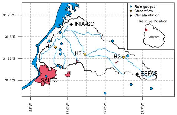 Figure 1
Hydrometeorological network and location of the San Antonio Catchment (225 km2)
Figure 1
Hydrometeorological network and location of the San Antonio Catchment (225 km2)
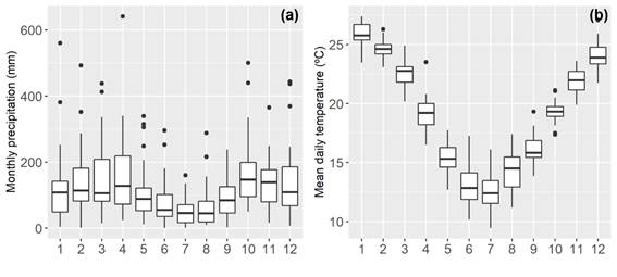 Figure 2
(a) Monthly precipitation and (b) mean daily
temperature at INIA-SG (1991-2020)
Figure 2
(a) Monthly precipitation and (b) mean daily
temperature at INIA-SG (1991-2020)
The relief of the San Antonio Catchment is characterized by rolling landscapes and plains that favor relatively slow runoff and drainage processes (Figure 3a). The hydrogeology is described by sedimentary deposits and fissured effusive rocks of Cretaceous-Tertiary periods which belong to the Salto-Arapey aquifer. The soils are Argiudolls & Hapluderts predominated by silty clay-silty clay loam(13). The main field capacity (Figure 3c) of the soils ranges 60-170 mm(14). The land use and land cover have not changed significantly in the last 10 years. The land use and land cover map of 2011(15) shows that the main land uses are row crops (46.6%), native forest (19.4%), herbaceous (11.7%), urban areas (11.8%), citrus trees (9.4%), and forestry (1.2%). This information forms the basis for creating the static input maps of the model (section 2.2). In addition, precipitation is preprocessed by interpolating daily precipitation using inverse distance weighting. This technique accounts for the spatio-temporal variability of precipitation and produces the dynamic input map of the model. Figure 3d shows an example of precipitation interpolation for a single convective event that occurred on September 8, 2019.
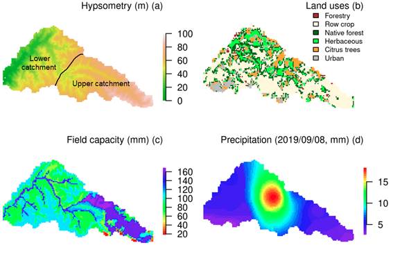 Figure 3
(a) Hypsometry, (b) land uses, (c) field
capacity, and (d) 24 h precipitation field for a single event in the San
Antonio Catchment
Figure 3
(a) Hypsometry, (b) land uses, (c) field
capacity, and (d) 24 h precipitation field for a single event in the San
Antonio Catchment
2.2 Rainfall-runoff model
The Hydrologiska Byråns Vattenbalansavdelning (HBV) model, developed by Sten Bergström at the Swedish Meteorological and Hydrological Institute(16)(17)(18), is one of the most widely used hydrological models worldwide(19). HBV is originally a daily lumped hydrologic model that uses precipitation and potential evapotranspiration as meteorological forcing (optionally, temperature is used to model snowmelt). Runoff, soil moisture, interception and infiltration are calculated at the catchment scale with few parameters. There are many versions of the model created over the years in different programming languages, such as Python, Matlab, R, Fortran(20)(21)(22)(23).
The SanAntonioApp uses the distributed version of the HBV-96 model(18) within the hydrologic modelling framework wflow (WFLOW-HBV) running in the Phyton environment(24). WFLOW-HBV has 4 components: (1) snow, (2) soil moisture, (3) sub-basin routing, and (4) river routing. The first component is not considered because there is no snow precipitation in the catchment (humid subtropical climate). The second component produces the soil water balance at a daily time step and provides the direct runoff. This routine also calculates infiltration, seepage and actual evaporation without time delay. Three types of runoff are then considered: quick runoff, interflow and slow runoff. The quick runoff and interflow are represented by a single linear reservoir with two outputs governed by the water content of the upper zone. Slow runoff is also represented by a linear reservoir and simulates exfiltration from the lower zone. Finally, the direct runoff is routed by the kinematic wave equation (river routing component) rather than the triangular unit hydrograph of the original HBV-96(25). In this approach, the hydraulic section of the river is partitioned by a main channel and floodplains (assumed to be rectangular channels). This configuration allows simulating fast flows in the mean channel and slow flow of the flood plains; this characteristic is due to high roughness and shallower depth of the flood plains with respect to the main channel. Equations and model diagrams can be found in the openstreams/wflow site(24).
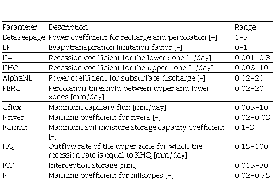
The spatial structure of the San Antonio WFLOW-HBV model divides the catchment into 5491 grid cells with a size of 0.002º (~200 m). The model runs for each cell at the daily scale using the dynamic input dataset (precipitation and potential evapotranspiration) and the static inputs maps (hypsometry, field capacity and land use) (section 2.1). The dynamic input dataset is the climatological forcing and the static input maps is used to parameterize each cell of the model; e. g., field capacity is related with soil type, a parameter that controls water storage in the soil. Then, the parameters of the model are optimized to improve the model performance (section 2.3). The description of the model parameters and the parameters ranges used in the sensitivity analysis are listed in Table 1.
Table 1
Parameters of the WFLOWHBV model and parameter ranges used in the sensitivity analysis
|
Parameter
|
Description
|
Range
|
|
BetaSeepage
|
Power coefficient
for recharge and percolation [-]
|
1-5
|
|
LP
|
Evapotranspiration
limitation factor [-]
|
0-1
|
|
K4
|
Recession
coefficient for the lower zone [1/day]
|
0.001-0.3
|
|
KHQ
|
Recession
coefficient for the upper zone [1/day]
|
0.006-10
|
|
AlphaNL
|
Power coefficient
for subsurface discharge [-]
|
0.02-20
|
|
PERC
|
Percolation
threshold between upper and lower zones [mm/day]
|
0.02-20
|
|
Cflux
|
Maximum
capillary flux [mm/day]
|
0.005-10
|
|
Nriver
|
Manning
coefficient for rivers [-]
|
0.02-0.03
|
|
FCmult
|
Maximum soil moisture
storage capacity coefficient [-]
|
0.1-3
|
|
HQ
|
Outflow rate of
the upper zone for which the recession rate is equal to KHQ [mm/day]
|
0.15-100
|
|
ICF
|
Interception
storage [mm]
|
0.015-30
|
|
N
|
Manning
coefficient for hillslopes [-]
|
0.02-0.75
|
2.3 Optimization of the model parameters
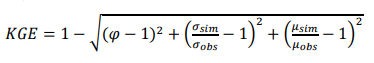
Optimization of model parameters (also known as model calibration) is performed to improve model results with respect to observed time series of streamflow. The goodness of fit of the model is quantified using the Kling-Gupta efficiency (KGE, Equation 1). This index accounts for correlation, bias and variability between model simulations and observations, and improves on other classical efficiency index such as Nash-Sutcliffe efficiency or mean squared error(26)(27).
Where φ is the Pearson
product-moment correlation coefficient; σ is the standard deviation of
simulations (sim) and observations (obs), and μ is the mean value of
simulations and observations. KGE ranges between -∞ and 1, values of KGE greater
than -0.41 indicate that the model improves the mean flow as a benchmark(28). KGE is chosen instead
of other objective functions that offer better fit at low flow rates(29), because we aim to obtain
the best possible fit over the full range of flows.
Before the optimization procedure, a General Sensitivity Analysis is performed by Latin Hypercubes Sampling (GSA-LHS) with 1000 samples to simplify and reduce the parameter space of the model. This technique is based on Markov Chain Monte Carlo (MCMC) experiments and allows ranking the parameters according to their importance(30)(31)(32), i. e., the model parameters with minor effect on the model results can be considered as constant values. Next, the optimization algorithm follows the Generalized Likelihood Uncertainty Estimation (GLUE)(33), which is based on the concept of equifinality and is associated with predictive uncertainty(34). In this technique, two groups of parameters/simulations are defined: behavioral denotes the group of parameters/simulations that are retained, and non-behavioral denotes the parameters/simulations that are discarded because they do not meet a minimum model performance criterion (defined by the objective function). GLUE also employs an MCMC sampling algorithm. For this purpose, a self-developed R script is coupled with the Python code WFLOW-HBV.
Model verification (also known as model validation) is made by internal spatial cross-validation(35) instead of the classical technique based on partitioning the time domain. In this technique, two of the three streamflow stations are used to optimize the parameters and one streamflow station is used to evaluate the model performance across ungauged sites. Internal spatial cross-validation takes advantages of multiple streamflows stations and minimizes the impact of a relatively short time period (July 2018 - February 2021).
2.4 Flow Duration Curves estimation
The Flow Duration Curves (FDC), as mentioned earlier (Section 1), is a cumulative frequency curve that indicates the percentage of time (or probability) that a given streamflow is equaled or exceeded during a given period. This curve is calculated with long-records of streamflow. In the absence of long-records of streamflow the FDC is produced by hydrologic simulation that provides predictions for ungauged sites. In this study, the distributed model WFLOW-HBV is used, which was spatially cross-validated over a relatively short period of time (3 years), which is not sufficient to produce a robust estimate of FDC. Considering this limitation, the time domain of the model was extended to a 30-year period (1991-2020), using the long-record of climate stations as the climatological forcing.
After the model simulations are performed for the long period, the FDC for each river cell is calculated with the complement of the cumulative distribution function of daily streamflow. Then, the FDC is considered as a step function, which can be calculated with equation 2, as follows:
Here FDC is the Flow Duration Curve for a given streamflow qx within a given period qt, the function num (qx,qt) counts the number of times were qt is less than qx, and n is the length of qt. Then, the monthly FDCs are obtained by arranging the model simulations by month.
3. Results
In this work, WFLOW-HBV model was implemented in the San Antonio catchment during the period July 2018 - February 2021 to estimate FDC in a distributed manner. The model was simplified from 12 to 5 parameters by GSA-LHS and optimized according to GLUE. In addition, the model was cross-validated in the inner spatial domain of the catchment. The FDCs were obtained by extending the simulation period to 1991-2020 using the long records of the climate stations. Finally, the results are stored in an R package SanAntonioApp and made available on the Github platform(10).
3.1 WFLOW-HBV setup and performance
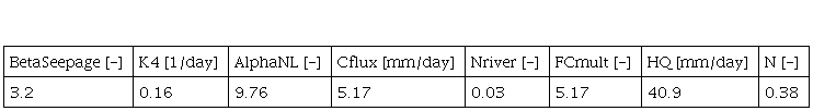
The GSA-LHS reveals that KGE is sensitive only to 4 of the 12 parameters of the model. The parameters ranked by the sensitivity index are: PERC (0.49), KHQ (0.29), LP (0.24), ICF (0.23), N(0.16), HQ (0.16), BetaSeepage (0.10), K4 (0.09), Nriver (0.07), FCmult (0.07), AlphaNL (0.05), Cflux (0.04), where the sensitivity index is the number between the parenthesis. The first 4 parameters are kept for optimization, while the other 8 are considered as constant values. This consideration is made to simplify the complexity of the optimization algorithm and to speed up the convergence. The values used for the parameters considered constant were obtained from the best 100 simulations of the GSA-LHS; these values are listed in Table 2.
Table 2
Values of parameters assumed as constant
|
BetaSeepage [-]
|
K4 [1/day]
|
AlphaNL [-]
|
Cflux [mm/day]
|
Nriver [-]
|
FCmult [-]
|
HQ [mm/day]
|
N [-]
|
|
3.2
|
0.16
|
9.76
|
5.17
|
0.03
|
5.17
|
40.9
|
0.38
|
Then, the PERC parameter was regionalized for the so-called “upper-catchment” (PERC1) and “lower-catchment” (PERC2). This regionalization was done to optimize the parameter according to the soil type, since the Field Capacity map shows that the upper-catchment differs from the lower-catchment (Figure 3c). The probability density functions of the behavioral parameters (Figure 4) show that PERC ranges from 0 to 10 mm (Figure 4a). The mean value of PERC1 is 5.5, while PERC2 is 3.2. The standard deviation of PERC1 and PERC2 is quite similar and is 2.4. KHQ has a behavioral response for the entire range of the sample domain (Figure 4b), with the most frequent behavioral values located around 7. ICF (Figure 4c) and LP (Figure 4d) are both slightly left skewed, with the mean of ICF being 22 mm and of LP being 0.8 (with the median values close to the mean in both cases).
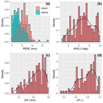 Figure 4
WFLOW-HBV optimized density functions of: (a) Percolation threshold for the
upper (PERC1) and lower (PERC2) catchment; (b) Recession coefficient for the
upper zone; (c) Interception storage, and (d) Evapotranspiration limitation
factor
Figure 4
WFLOW-HBV optimized density functions of: (a) Percolation threshold for the
upper (PERC1) and lower (PERC2) catchment; (b) Recession coefficient for the
upper zone; (c) Interception storage, and (d) Evapotranspiration limitation
factor
The KGE values are greater than 0.7 after the optimization/validation procedures, H1 has better performance than H2, and H2 has better performance than H3 (Figure 5a). In other words, the performance of the model decreases as the area of the sub-basins increases. The percentage of bias (Figure 5b) is 10% with under/over-estimate for the lower/upper zones of the catchment. Internal spatial cross-validation is performed only for H2 and H3. This consideration was made to avoid the singularities of the lower catchment; for example, the lower catchment has field capacities below 100 mm, while the upper catchment is in the range of 60-170 mm (Figure 3c). The validation procedure shows that the performance of the model is retained for the inner spatial domain with a small loss of prediction skill.
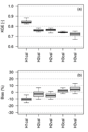 Figure 5
(a)
Kling-Gupta Efficiency (KGE) and (b) Percentage Bias of model simulations on
H1, H2 and H3 streamflow stations (subindex cal &
val mean calibration and validation, respectively)
Figure 5
(a)
Kling-Gupta Efficiency (KGE) and (b) Percentage Bias of model simulations on
H1, H2 and H3 streamflow stations (subindex cal &
val mean calibration and validation, respectively)
Figure 6 shows a graphical verification of the observed and simulated hydrographs for January 2019. This month was an extraordinarily rainy month with multiple complex flood events that are particularly difficult to simulate. The black lines represent the observed runoff, the red line is the mean of the behavioral simulations, and the grey shadow is the 95% prediction uncertainty. The ratios of January 2019 maximum streamflows to calibration period maximum streamflows are 0.56 (Chico), 0.42 (Cabecera) and 0.34 (Ruta 3). This graphical representation shows that the peaks streamflows are well represented with a slight delay for a few days. An interesting aspect for stations H2 and H3 is that the observed values show 5 streamflow peaks rather than the 4 simulated peaks given by WFLOW-HBV.
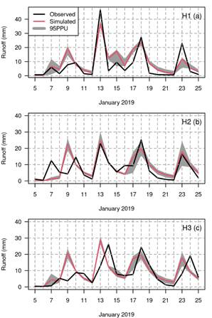 Figure 6
Observed and simulated hydrographs for January
2019 with the 95% prediction uncertainty (95PPU) for (a) H1, (b) H2, and (c) H3
streamflow stations
Figure 6
Observed and simulated hydrographs for January
2019 with the 95% prediction uncertainty (95PPU) for (a) H1, (b) H2, and (c) H3
streamflow stations
3.2 Flow Duration Curves
Monthly and annual Flow Duration Curves have been estimated for the entire river domain. Figure 7 shows the FDC for August (Figure 7a), October (Figure 7b), and April (Figure 7c) for an arbitrary river section of the river located at -57.829ºW -31.307ºS (blue lines) and the annual FDC (red lines). This figure can be read according to two basic interpretations: (1) Shifted curves, when one curve is shifted to the left relative to the other low streamflow will be more frequent. This is the case for August and October, where August (shifted to the left with respect to annual) is generally below the annual streamflow and annual streamflow is below October (shifted to right with respect to annual). (2) Looped curves, this is an interesting case that shows differences in the variance of the two datasets. For example, April is below annual on the left-tail, and above on the right-tail. This means that both high and low streamflows are more common in April. Also, the interception of the two curves implies equal probability for a given streamflow. Another view is obtained by contrasting the probability density distributions of the streamflow which show the probability within a certain range (Figure 7d-f). This representation shows shifted to the left for August, shifted to the right for October, and high dispersion and flattening for April, which is helpful in interpreting the FDC.
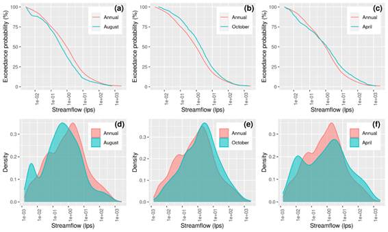 Figure 7
(a-c)
Monthly Flow Duration Curves and (d-f) Monthly Density probability distribution
of daily streamflow for an arbitrary river section located in -57.829ºW
-31.307ºS
Figure 7
(a-c)
Monthly Flow Duration Curves and (d-f) Monthly Density probability distribution
of daily streamflow for an arbitrary river section located in -57.829ºW
-31.307ºS
3.3 SanAntonioApp
FDC were shared with the SanAntonioApp R package(10). The package is hosted on the Github platform and can be installed via the R console by the following command:
devtools::install_github("rafaelnavas/SanAntonioApp")
The package has been tested on Ubuntu and Windows operating systems. Version 1.0. contains the folder “data”, with the FDCs and the function “SanAntonioFDC()”, which runs the application into your local environment. In addition, to make the application available from any browser, it is temporarily placed in the following link: https://rafaelnavas23.shinyapps.io/SanAntonioApp/.
The SanAntonioApp allows the user to query the FDC by month and location. The month is selected by the user with a slider input, and the locations are selected by a simple click on the map. The input panel is located on the left side under the tag “Aplicación”. The FDC is then displayed on the right side of the screen. Figure 8 shows a simplified display of the application.
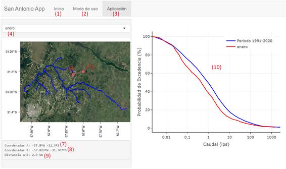 Figure 8
Display of the SanAntonioApp: The bottom “Inicio” (1) is the home with credits. Brief instructions
are shown in “Modo de uso” (2). The application page
can be accessed by clicking “Aplicación” (3). The
month can be chosen in the slider input (4). Location of the target site is
assigned by clicking on the map. (6) Location of estimation site, (7) Coordinates
of the target site, (8) Coordinates of the estimation site, (9) Distance
between target and estimation sites, (10) Flow Duration Curve
Figure 8
Display of the SanAntonioApp: The bottom “Inicio” (1) is the home with credits. Brief instructions
are shown in “Modo de uso” (2). The application page
can be accessed by clicking “Aplicación” (3). The
month can be chosen in the slider input (4). Location of the target site is
assigned by clicking on the map. (6) Location of estimation site, (7) Coordinates
of the target site, (8) Coordinates of the estimation site, (9) Distance
between target and estimation sites, (10) Flow Duration Curve
4. Discussion
Spatially distributed FDC were estimated for the San Antonio catchment. Estimation was performed by distributed hydrological simulation using the WFLOW-HBV model. The conceptual model of the catchment represents the actual physical properties shown in Figure 3. In other words, the model does not take into account land use changes, farmer-led irrigation development or climate change; which are factors that could have an effect in the runoff response of the catchment(36)(37)(38). According to the land use map of 2000, and information given by the National Water Authority (DINAGUA), there has been no significant change in land use or surface water allocation in the catchment over the past 20 years, which gives some confidence to the hypothesis taken in the model implementation.
Some applications of the FDC can be summarized as: (1) estimating water quantity and frequency in the interior of the catchment. This is useful for knowing whether a section of river can meet a particular water demand. For example, a farmer on the riverbank might know how much water is available and how often that amount is guaranteed. (2) Environmental flow estimation. A variety of definitions of environmental flow can be found in the literature. Basically, it is the flow regime required to achieve the desired ecological objectives. Look-up tables, desktop analysis, functional analysis and hydraulic habitat modelling are different approaches used around the world(39). In Uruguay, environmental flow is determined using look-up tables in the Decree 368/018 (provisional)(40), which determines environmental flow based on the probability of exceeding the daily streamflow for a given month, location in the river, and the type of water intakes. The preliminary regulation establishes an exceedance probability of 60% for reservoirs and 80% for direct water intake. These values of streamflow can be easily determined at any location in the catchment using the SanAntonioApp.
An interesting finding in the optimization of the distributed model was that the performance of the model decreases as the area of the sub-basins increases. These results contradict previous research that found that catchments with larger areas generally performed better(30)(41). However, this finding could be explained by the fact that the uncertainty in the hydrologic simulation also depends on the uncertainty in the precipitation input(42)(43)(44). The present study was conducted with a very high density of rain gauges for the lower catchment (Figure 1). The rain gauge network design had two purposes: (1) to validate rainfall estimation using microwave links(45), which requires a large number of rain gauges in a very small area, and (2) calibration/validation of the hydrologic model used in the present study. This fact explains why the upper part of the basin may be subject to larger uncertainties in the precipitation input. In addition, the model in the lower/upper catchment shows a negative/positive bias. This result could be due to the dynamics between the aquifer and surface waters, which is mainly dominated by percolation in the upper catchment and exfiltration in the lower catchment, which is not considered by the model. Another source of uncertainty are the dynamics of vegetation, which affects actual evapotranspiration, and the influence of climate variability(46)(47). Neither factor was considered in this work. Future works should study the implementation and performance of integrated surface-subsurface models(48) and the testing of information content given the dependence of parameter to climate variability.
The FDC generated in the present study allows to characterize the streamflow regime by month, with August being the month with less streamflow, and October and May being the months with more streamflow. In addition, April is more variable than the other months. This hydrological regime is triggered by precipitation, which has a similar shape. The streamflows regime in the San Antonio catchment in northern Uruguay contrasts with the hydrological regime of some basins in the south of the country. For example, the hydrologic regime of the Santa Lucia catchment is mainly determined by temperature/evapotranspiration, since precipitation is uniform throughout the year(37).
5. Conclusions
This paper presents the development of the SanAntonioApp, which is part of the project "Toward an Integrated Water Resources Management of Highly Anthropized Hydrological Systems: San Antonio Creek - Salto/Arapey Aquifer", funded by the National Agency for Investigation and Innovation.
The SanAntonioApp is an R package and application that contains the WFLOW-HBV model of the San Antonio catchment, the input dataset, model outputs and interactive visualization tools for Flow Duration Curves. The application can be used to estimate the frequency of a given flow or the flow for a given frequency at any location in the river network, which is useful for estimating water availability as well as environmental flows for current water regulation in Uruguay.
Acknowledgments
This publication was supported by the National
Agency for Investigation and Innovation, María Viñas Fund
– 2017 (FMV_1_2017_1_135656).
References
1. Arthington AH. Environmental flows: saving rivers in the third millennium. Berkeley: University of California Press; 2012. 424p.
2. Vogel RM, Fennessey NM. Flow‐duration curves: I. new interpretation and confidence intervals. J Water Resour Plan Manag. 1994;120(4):485-504.
3. Blöschl G, editor. Runoff prediction in ungauged basins: synthesis across processes, places and scales. Cambridge: Cambridge University Press; 2013. 465p.
4. Narbondo S, Gorgoglione A, Crisci M, Chreties C. Enhancing physical similarity approach to predict runoff in ungauged watersheds in sub-tropical regions. Water. 2020;12(2):528. doi:10.3390/w12020528.
5. Perrin C, Michel C, Andréassian V. Improvement of a parsimonious model for streamflow simulation. J Hydrol. 2003;279(1-4):275-89.
6. Pilgrim DH. Some problems in transferring hydrological relationships between small and large drainage basins and between regions. J Hydrol. 1983;65(1-3):49-72.
7. Arnold JG, Youssef MA, Yen H, White MJ, Sheshukov AY, Sadeghi AM, Moriasi DN, Steiner JL, Amatya DM, Skaggs RW, Haney EB, Jeong J, Arabi M, Gowda PH. Hydrological processes and model representation: impact of soft data on calibration. Trans ASABE. 2015;58(6):1637-60.
8. R Core Team. R: The R Project for Statistical Computing [Internet]. 2021 [cited 2022 Aug 22]. Available from: https://www.r-project.org/.
9. Slater LJ, Thirel G, Harrigan S, Delaigue O, Hurley A, Khouakhi A, Prosdocimi I, Vitolo C, Smith K. Using R in hydrology: a review of recent developments and future directions. Hydrol Earth Syst Sci. 2019;23(7):2939-63.
10. Navas R. rafaelnavas/SanAntonioApp: SanAntonioApp [Internet]. Zenodo. 2021 [cited 2022 Aug 22]. Available from: https://zenodo.org/record/5223882.
11. Peel MC, Finlayson BL, McMahon TA. Updated world map of the Köppen-Geiger climate classification. Hydrol Earth Syst Sci. 2007;11(5):1633-44.
12. World Meteorological Organization. Manual on stream gauging. Geneva: WMO; 2010. 2p.
13. Ministerio de Ganadería, Agricultura y Pesca, RENARE (UY). Mapa General de Suelos del Uruguay, según Soil Taxonomy USDA [Internet]. IDEUy. 2001 [cited 2022 Aug 22]. Available from: https://visualizador.ide.uy/geonetwork/srv/api/records/1335f1c8-65eb-46df-8fba-9310a338e692.
14. Molfino JH, Califra A. Agua disponible de las tierras del Uruguay. Montevideo: MGAP; 2001. 13p.
15. Ministerio de Vivienda y Ordenamiento Territorial (UY). Cobertura del suelo [Internet]. Montevideo: MVOTMA; 2011 [cited 2022 Aug 24]. Available from: https://sit.mvotma.gub.uy/geonetwork/srv/spa/catalog.search#/metadata/b8b30f73-67f8-4535-a505-9ac953984159
16. Bergström S. The HBV model: its structure and applications. SMHI Reports Hydrology [Internet]. 1992 [cited 2022 Aug 24];(4):32p. Available from: https://www.smhi.se/polopoly_fs/1.83592!/Menu/general/extGroup/attachmentColHold/mainCol1/file/RH_4.pdf
17. Bergström S. Development and application of a conceptual runoff model for Scandinavian Catchments. Norrköping: Sveriges Meteorologiska OCH Hydrologiska Institut; 1976. 162p. SMHI Rapporter.
18. Lindström G, Johansson B, Persson M, Gardelin M, Bergström S. Development and test of the distributed HBV-96 hydrological model. J Hydrol. 1997;201(1):272-88.
19. Wetterhall F. HBV – The most famous hydrological model of all?: An interview with its father: Sten Bergström. HEPEX [Internet]. 2014 Dec 16 [cited 2022 Aug 22]. Available from: https://hepex.inrae.fr/the-hbv-model-40-years-and-counting/
20. Craven J. Python implementation of the HBV Hydrological Model [Internet]. 2021 [cited 2022 Aug 22]. Available from: https://github.com/johnrobertcraven/hbv_hydromodel
21. HRL. HBV-EDU Hydrologic Model [Internet]. Version 1.0.0.0. 2021 [cited 2022 Aug 22]. Available from: https://www.mathworks.com/matlabcentral/fileexchange/41395-hbv-edu-hydrologic-model
22. Saelthun NR. The Nordic HBV Model [Internet]. [place unknown]: Hydrology Department; 1996 [cited 2022 Aug 22]. 27p. (Publication; nº 7). Available from: https://www.osti.gov/etdeweb/servlets/purl/515690
23. Toum E. HBV.IANIGLA: Modular Hydrological Model [Internet]. 2021 [cited 2022 Aug 22]. Available from: https://CRAN.Rproject.org/package=HBV.IANIGLA
24. Schellekens J, van Verseveld W, Visser M, hcwinsemius, laurenebouaziz, tanjaeuser, sandercdevries, cthiange, hboisgon, DirkEilander, DanielTollenaar, aweerts, Fedor Baart, Pieter9011, Maarten Pronk, arthur-lutz, ctenvelden, Imme1992, Jansen M. openstreams/wflow: Bug fixes and updates for release 2020.1.2 [Internet]. 2020 Nov 26 [cited 2022 Aug 22]. Available from: https://zenodo.org/record/593510
25. Schellekens J. The wflow_routing Model — wflow documentation [Internet]. Revision 2c69dde2. 2019 [cited 2022 Aug 22]. Available from: https://wflow.readthedocs.io/en/stable/wflow_routing.html
26. Gupta HV, Kling H, Yilmaz KK, Martinez GF. Decomposition of the mean squared error and NSE performance criteria: Implications for improving hydrological modelling. J Hydrol. 2009;377(1-2):80-91.
27. Kling H, Fuchs M, Paulin M. Runoff conditions in the upper Danube basin under an ensemble of climate change scenarios. J Hydrol. 2012;424-425:264-77.
28. Knoben WJM, Freer JE, Woods RA. Technical note: Inherent benchmark or not? Comparing Nash–Sutcliffe and Kling–Gupta efficiency scores. Hydrol Earth Syst Sci. 2019;23(10):4323-31.
29. Pushpalatha R, Perrin C, Moine NL, Andréassian V. A review of efficiency criteria suitable for evaluating low-flow simulations. J Hydrol. 2012;420-421:171-82.
30. Navas R, Delrieu G. Distributed hydrological modeling of floods in the Cévennes-Vivarais region, France: impact of uncertainties related to precipitation estimation and model parameterization. J Hydrol. 2018;565:276-88.
31. Hornberger GM, Spear RC. Approach to the preliminary analysis of environmental systems. J Environ Manage. 1981;12:7-18.
32. Gan Y, Liang XZ, Duan Q, Ye A, Di Z, Hong Y, Li J. A systematic assessment and reduction of parametric uncertainties for a distributed hydrological model. J Hydrol. 2018;564:697-711.
33. Beven K, Binley A. The future of distributed models: model calibration and uncertainty prediction. Hydrol Process. 1992;6(3):279-98.
34. Brazier RE, Beven KJ, Freer J, Rowan JS. Equifinality and uncertainty in physically based soil erosion models: application of the GLUE methodology to WEPP–the Water Erosion Prediction Project–for sites in the UK and USA. Earth Surf Process Landf. 2000;25(8):825-45.
35. Tegegne G, Park DK, Kim YO. Comparison of hydrological models for the assessment of water resources in a data-scarce region, the Upper Blue Nile River Basin. J Hydrol Reg Stud. 2017;14:4966.
36. Aznarez C, Jimeno-Sáez P, López-Ballesteros A, Pacheco JP, Senent-Aparicio J. Analysing the impact of climate change on hydrological ecosystem services in Laguna del Sauce (Uruguay) using the SWAT model and remote sensing data. Remote Sens. 2021;13(10):2014. doi:10.3390/rs13102014.
37. Navas R, Alonso J, Gorgoglione A, Vervoort RW. Identifying climate and human impact trends in streamflow: a case study in Uruguay. Water. 2019;11(7):1433. doi:10.3390/w11071433.
38. Silveira L, Gamazo P, Alonso J, Martínez L. Effects of afforestation on groundwater recharge and water budgets in the western region of Uruguay. Hydrol Process. 2016;30(20):3596-608.
39. Acreman MC, Dunbar MJ. Defining environmental river flow requirements?: a review. Hydrol Earth Syst Sci Discuss. 2004;8(5):861-76.
40. Aprobacion de medidas para que los usos de las aguas publicas aseguren el caudal que permita la proteccion del ambiente y criterios de manejo ambientalmente adecuados de las obras hidraulicas. Decreto N° 368/018 [Internet]. 2018 [cited 2022 Aug 22]. Available from: https://www.impo.com.uy/bases/decretos/368-2018
41. Arnaud P, Lavabre J, Fouchier C, Diss S, Javelle P. Sensitivity of hydrological models to uncertainty in rainfall input. Hydrol Sci J. 2011;56(3):397-410.
42. Germann U, Berenguer M, Sempere-Torres D, Zappa M. REAL-Ensemble radar precipitation estimation for hydrology in a mountainous region. Q J R Meteorol Soc. 2009;135(639):445-56.
43. Habib E, Aduvala AV, Meselhe EA. Analysis of radar-rainfall error characteristics and implications for streamflow simulation uncertainty. Hydrol Sci J. 2008;53(3):568-87.
44. Kavetski D, Kuczera G, Franks SW. Bayesian analysis of input uncertainty in hydrological modeling: 1. Theory. Water Resour Res. 2006;42(3). doi:10.1029/2005WR004376.
45. Sapriza-Azuri G, Gamazo P, Erasun V, Banega R, Poses A, Navas R, Alcoba M, Gosset M. Rainfall estimation by microwave links in Uruguay: first results. Geophys Res Abstr [Internet]. 2019 [cited 2022 Aug 22];21:EGU2019-5229. Available from: https://meetingorganizer.copernicus.org/EGU2019/EGU2019-5229.pdf.
46. Osuch M, Romanowicz RJ, Booij MJ. The influence of parametric uncertainty on the relationships between HBV model parameters and climatic characteristics. Hydrol Sci J. 2015;60(7-8):1299-316.
47. Ala-aho P, Soulsby C, Wang H, Tetzlaff D. Integrated surface-subsurface model to investigate the role of groundwater in headwater catchment runoff generation: a minimalist approach to parameterisation. J Hydrol. 2017;547:664-77.
48. Jayathilake DI, Smith T. Understanding the role of hydrologic model structures on evapotranspiration-driven sensitivity. Hydrol Sci J. 2020;65(9):1474-89.
Author notes
rafaelnavas23@gmail.com
Additional information
Editor: Mónica M. Barbazán https://orcid.org/0000-0002-5501-064X Universidad de la
República, Facultad de Agronomía, Montevideo, Uruguay
Author contribution statement: RN designed the analysis and wrote the
paper. VE and RB carried out the experiments and helped to write the manuscript.
GS conceived and planned the experiments, and provided critical feedback to the
manuscript. AS conducted data analysis. PG supervised the project.
Alternative link
http://agrocienciauruguay.uy/index.php/agrociencia/article/view/979/1273 (pdf)


 [Equation 1]
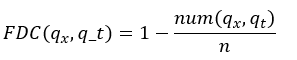 [Equation 2]

