I. INTRODUCTION

Throughout history, Ecuador has based its trade policy on being a primary producer and exporter. At the same time, being an unindustrialized country, it has been an importer of consumption goods and very little of capital goods for its respective input processing. On the other hand, Ecuador has traditionally had a closed economy behavior. To corroborate this information, the Global Edge Portal of the State University of Michigan (2017) classifies Ecuador as 60 out of 135 as an exporter, 69 out of 134 as importer, and 33 out of 134 in the trade balance. This shows the country's little impact on international trade.

However, in the 1970s, the oil boom and returning to democracy -after a long period of military dictatorship- caused a very significant increase for the Ecuadorian international trade, whose oil began to be exported in huge amounts and thus generating a considerable income of foreign exchange (Behar & Nelson, 2014). For this last reason, it is decided to delimit the present research work from the year 1970 to 2015.

From that decade on, oil is so important to the Ecuadorian economy that foreign trade bulletins discriminate exports, imports, and oil and non-oil trade balance. Throughout these four decades, all periods have recorded deficits in non-oil trade balances confirming Ecuador's high oil dependence on its international trade relations.

Moreover, according to the World Trade Organization, Ecuador is in position 69 and 80 for exports and imports, respectively, in the ranking of merchandise trade, from a total of 135 countries. And its portion of trade in comparison with its GDP was 23.6% for 2015. Nowadays, Ecuador plays a more relevant role in the international trade. In fact, the World Trade Organization (WTO) considered Ecuador as the world’s leading exporter of bananas, hearts of palm, and roses, and the third largest exporter of flowers.

Once the Ecuadorian foreign trade scenario has been expressed, this research work has as its main objective the analysis of Ecuador's insertion in globalization by measuring the openness it has had to international trade with other countries and how it has gone evolving over time, using some estimates and models that will help us to understand this evolution of Ecuadorian foreign trade from a more technical point of view.

From this and to cover with the outlined goal, the present research work has been divided into different sections. The first section is a descriptive analysis of Ecuadorian foreign trade such as its main exported and imported products, the main destinations and origins of the products it sells. Then, it moves to the methodological part of the work. In this research it has been decided to use different estimations of the gravity model: Ordinary Least Squares (OLS), country pair fixed effects (CPFE), the Hausman Taylor model (HT), and the Pseudo Poisson Maximum Likelihood Estimation (PPML). This section presents a brief description of its main concepts, features and advantages of each estimation model.

After presenting the data, the next section encapsulates the presentation and interpretation of the results obtained from the different models used. A table with the results of the OLS regression, fixed effects and Hausman Taylor models will be presented. Then, we use the coefficients obtained with the Hausman estimator in order to make a comparison between real and predicted exports (and imports) for the ten main destinations (and origins) to determine if Ecuador has been opening to trade and inserting itself in globalization, i.e., if real trade has been exceeding the predicted one.

Moreover, the main results of the PPML estimation with its respective interpretation will be presented, as well as an analysis of the impact that dollarization and forming part of the Andean Community have had in the Ecuadorian international trade. Finally, the main conclusions of the work are presented.

II. ECUADORIAN’S TRADE POLICY OVERVIEW

The current section presents the evolution of exports, imports and trade balance over time, as well as the level of exports and imports with the ranking of the top ten business partners. In addition, the main types of products exported and imported in recent years are presented. In the following paragraphs, a description and analysis of the evolution of Ecuador's international trade will be presented in order to understand its behavior and its insertion in globalization.

Exports

According to the Ministry of Foreign Trade of Ecuador, exports grew by 14% in 2015 compared to the previous year. The United States continues to be the main destination for exports, followed by the European Union and Vietnam. These three markets represent 56% of total of Ecuadorian exports (Ministerio de Comercio Exterior e Inversiones del Ecuador, 2014).

For the Ecuadorian economy, oil has been its main product sold for around four decades. For this reason, it is usual to discriminate exports into oil and non-oil. As for oil companies, the sale of crude accounted for 8% growth in relation to 2014. Regarding non- oil companies, for 2015, 71% of these consisted in shrimp (with 18% growth), bananas (11%), canned fish (29%), natural flowers and cocoa

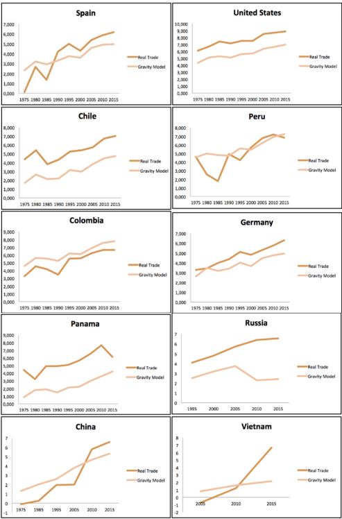
According to the World Trade Organization, the ten main destinations of Ecuadorian products, currently, are: United States, Chile, Vietnam, Peru, Colombia, Russia, Panama, China, Spain and Germany. It has taken the ten main partners at the present, in order to analyze the behavior of Ecuador's trade relations with them through history. The following chart shows the evolution of exports with these ten trading partners since 1970.

Figure 1 shows each of the ten best partners for Ecuadorian exports, clustered by decades. Thus, the Figure let us conclude with several points: from decades before 2000-2009, only the US accumulated close or more than ten billion of Ecuadorian goods purchases. This means that, before 2000, Ecuador seemed to have a closed economy identity, despite the oil boom and the return to democracy. It is from 2000 when really begins to have positive peaks. It should be noted that after 2000, the dollar became the official currency.

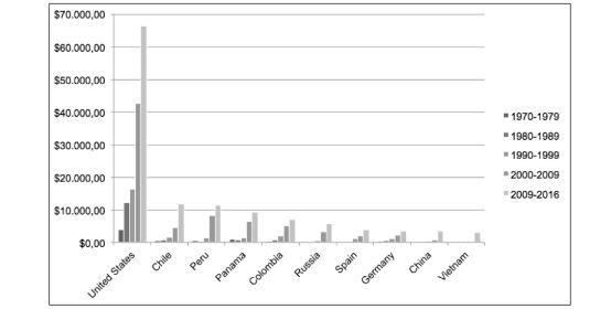Figure 1
Main destinations of exports 1970-2015
Source: International Monetary Fund Elaboration: Author

Another point is the emergence of new important partners for Ecuador (such as Vietnam, China, Spain, Germany, or Russia), which until 2000 decade the level of Ecuadorian exports was reaching zero and now reaches almost 2000 million on average and in cases as Peru or Panama reached a cumulative of close to 10 billion dollars. This emergence of new relevant business partners has occurred, in large part, due to several trade agreements signed by governments, which will be analyzed in the next section.

According to the Ministry of Foreign Trade of Ecuador, currently, the main exported products are: oil, shrimp, bananas, canned fish, natural flowers, cocoa, extracts and vegetable oils, other metal manufactures, other woods, gold, and fish. Figure 2 shows the high dependence on primary products in Ecuadorian exports. In fact, only using as reference the period from 2013 to 2015, a total of 104,726 million dollars was registered of which 83,605 represent primary products and only 21,120 industrialized products. Below is an analysis of exports by product types: primary and industrialized.

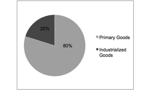Figure 2
Exports by type of products
Source: International Monetary Fund Elaboration: Author Ecuador and its insertion in glob

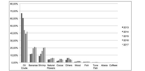Figure 3
Primary Goods Exports 2013-2015
Source: International Monetary Fund Elaboration: Author

Figure 3 shows the proportion of each type of good with respect of total of primary goods exports of the year. Apparently, crude oil has gone down from year to year with respect to the previous one, starting in 2014 it began to decrease and continued to decrease until 2015, which had a slight recovery in exports. On the other hand, products such as bananas and shrimp have had significant growth year after year, representing (on average) between 15 and 20% of total primary exports.

On the other hand, in Figure 4 it is shown the proportion of each type of good with respect to the total of industrialized goods exports of each year. Only the main products will be mentioned, which are: petroleum derived products, products made from coffee, products made from cocoa, fishmeal, and so on.

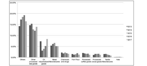Figure 4
Industrialized Products Exports 2013-2015
Source: International Monetary Fund Elaboration: Author

According to Figure 4, an important point is that ‘processed marine products’ is the main exporter sector₁ and have had an increasing and decreasing trend year after year, representing average between 12 and 15% of the total. Moreover, oil industrialized products in 2014 had a fall due to the collapse in crude oil prices but the rest of the year has had a growth trend. At this point it should be noted that although crude oil is exported as a primary good and represents between 60 and 65% of total primary exports, products processed from crude do not exceed 15%, showing the deficiency and little technology endowment in the country.

Imports

According to the Ministry of Foreign Trade of Ecuador, in 2015 the total amount of imports grew by 22% compared to 2014. Consumer goods were those with the highest increase (31%) followed by fuels and lubricants (28%), capital goods (19%), and raw materials (18%). Non-oil imports grew by 21%. China ranked first as the origin of imports with an annual growth of 19%, followed by the European Union (25%), the United States (11%), Colombia (21%), and Brazil (29%) (Ministerio de Comercio Exterior e Inversiones del Ecuador, 2015).

According to the World Trade Organization, the ten main origins of Ecuadorian purchases are the United States, China, Colombia, Brazil, Peru, South Korea, Mexico, Panama, Japan, and Germany. It has taken the ten main partners of the present for analyzing the behavior of Ecuador's trade relations with them since 1970. The following Figure shows the evolution of imports with these ten trading partners throughout history.

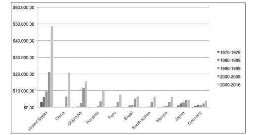Figure 5
Main origins of imports 1970-2015
Source: International Monetary Fund Elaboration: Author

Figure 5 shows each of the top ten partners for Ecuadorian imports, clustered by decades. From decades before 2000-2009, only the US accumulated close or more than ten billion of Ecuadorian goods purchases. Until the 90s, imports did not exceed ten billion CIF dollars per decade. From then on, imports rose, except for 1999 and 2000, which, given the banking crisis that the country went through and the definitive exchange of currency, caused imports to fall sharply.

In addition, and in parallel with exports, the great contribution that the United States has represented throughout the period under study is very evident. The participation of China at the end of the period as a major supplier of consumer and capital goods in Ecuador is also a quite relevant point. It is also worth noting the participation of neighbors Colombia and Peru since 1970, and the emergence of new suppliers that year after year increase commercial relations with Ecuador, such as Panama, South Korea, Japan and Germany.

Moreover, Panama and Colombia exceeded the ten billion for the last decade, and China and the US twenty billion for Ecuadorian foreign goods purchases. Actually, the US almost reached the fifty billion accumulated during the last decade. This shows the high significance that the US has for Ecuadorian imports.

According to the Chamber of Commerce of Quito, within the groups of products, the main imported between 2013 and 2015 were: raw materials representing 33% of total, capital 26%, consumer goods 21%, and fuels 20%. This allows us to conclude in several points: industrialized goods represent 41% of total and the imports of technology and commodities represent the remaining 59%. This shows us how little industrialized the country is and that it has always depended on industrialized products. This panorama has changed with respect to previous years (65% processed goods, 35% capital goods and raw materials) given the previous government program called "Change in the productive matrix" where incentives were created to technify and process goods locally (Cámara de Comercio de Quito, 2018).

Paradoxically, despite the high volume of exports of crude oil, the level of imports of petroleum products is very high, due to the lack of technology for the processing of crude oil and so that higher revenues can be obtained from processed exports. Given the limitation that imported products vary throughout history, it has also been difficult to collect data for all years, and it is also considered more relevant to include the current ones, therefore an analysis of both oil and non-oil imports of the most significant products will be presented.

The Figure 6 shows the imports by economic classification of products by use or economic destination. The amounts of imports are shown in percentage of each group with respect of total amount of imports.

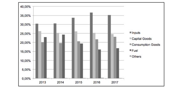Figure 6
Imports by Economic Classification of Products by Use or Economic Destination 2013-2015
Source: Chamber of Commerce of Quito.

There are some points to highlight. The import of consumer goods has remained between 19 and 23% of the total, having a tendency of growth and decrease year by year. In addition, the import of fuels only in 2013 and 2014 exceeded 20% of the total, from there the trend was always downward, having a slight recovery in 2015, representing 17% of the total.

On the other hand, inputs have had a growth trend (except for 2015) and have represented between 30 and 37% of the total between 2013 and 2015. Likewise, they have had a balanced trend, with growths and decreases, but within of 23 and 26% of total exports. These two groups represent between 55 and 60% of the total imports that would be destined for the processing of the primary goods and that however the export of the industrialized ones is quite low, supposing a deficiency in the endowment of technology and that could be object of study in future research.

III. METHODOLOGY

Gravity Model

In the area of international trade relations, the Gravity Model has been used to calculate the effect of alliances and treaties on commercial activities. The model has also been used to analyze the effectiveness of trade agreements and organizations, such as the World Trade Organization and the North American Free Trade Agreement. The gravity model of trade has been a success from the empirical point of view (Chaney, 2018)

The gravity model in international trade is similar to other models of gravity in the social sciences and it predicts bilateral trade flows based on economic sizes (generally the GDP of each economy) and the distance between them. Trade flows have also other determinants, such as common borders, common languages, common legal systems, common currencies or common colonial legacy. The analysis of these determinants is the main objective for the application of the gravity model (Kimura & Lee, 2006).

As applications of gravity models grow, there has been persistent research on the theoretical foundations of gravity models. Anderson (1979) and Anderson and van Wincoop (2003) provide the first and last more relevant examples of that. Currently, the gravity model has solid foundations on well-known theories, and its wide applicability in the prediction of socio-economic interactions does not surprise geographers and other social scientists (Henao-Rodríguez, Lis-Gutiérrez, Viloria, & Ariza, 2016).

Gravity in trade is related to the fact that larger economies tend to export and import more than the smaller ones. Moreover, economies that face higher levels of commercial costs tend to export and import less than those that face lower levels. Comparing with the basic model of gravity physics, trade is the "force" of economic attraction between two countries: one is pulling goods towards oneself from the other. The 'mass' in economic terms is approximately the GDP of a country. The distance between countries is taken as an indicator of the level of bilateral trade costs faced by transactions. Therefore, the basic gravity equation in international trade would be:

(1)

Where:

𝑋𝑖𝑗 is the value of trade between country i and country j

C is a constant

𝑌𝑖 the GDP of country i 𝑌𝑗

is the GDP of country j

𝐷𝑖𝑗 is the distance between country i and country j

Hence, the gravity model is commonly estimated as:

(2)

But as before noted, in equation 2, other variables can be relevant in international trade and must be taken into account when modeling gravity. For instance, cultural and historical affinity: if two countries have cultural ties, it is common that they also have strong economic ties. The variables generally used with this type are colonization, common language, common religion, and so on. In addition, geographic variables are also taken into account: if ocean ports facilitate trade, sharing a border can also reduce trade costs if compared to an isolated island that could increase them. Finally, it is relevant to include the members in economic integration agreements such as the Preferential Trade Agreements (PTAs), the Currency Union (CU), the GATT / WTO and Regional Trade Agreements (RTAs) in order to compute the effect of signing agreement in trade openness (Van Bergeijk & Brakman, 2010).

Fixed effects

The fixed-effect model allows correlating the unobserved individual effects with the included variables. Then we model the differences between units strictly as parametric changes of the regression function. This modeling expects that distinctions crosswise over units can be caught in contrasts in the constant term. Each 𝛼𝑖 is treated as an unknown parameter to be estimated. Let 𝑦𝑖 and 𝑋𝑖 be the N observations for the ith unit, i be a N × 1 column of ones, and let 𝜀𝑖 be associated N × 1 vector of disturbances. If 𝑧𝑖 is unobserved, but correlated with 𝑥𝑖𝑡, then the least squares estimator of β is biased and inconsistent as a consequence of an omitted variable. However, in this instance, the model

(2)

Where 𝛼𝑖 = 𝑧𝑖′𝛼, embodies all the observable effects and specifies an estimable conditional mean. This fixed effects approach takes 𝛼𝑖 to be a group-specific constant term in the regression model. It should be noted that the term “fixed” as used here indicates that the term does not vary over time, not that it is non- stochastic, which need not be the case (Greene, 2017).

Hausman-Taylor Estimation

The Hausman and Taylor (1981) model is a hybrid that combines the consistency of a fixed-effects model with the efficiency and applicability of a random-effects model. One-way random-effects models assume exogeneity of the regressors, namely that they be independent of both the cross-sectional and observation- level errors. In cases where some regressors are correlated with the cross-sectional errors, the random effects model can be adjusted to deal with endogeneity. The Hausman-Taylor estimator is an instrumental variables regression on data that are weighted similarly to data for random-effects estimation. In both cases, the weights are functions of the estimated variance components (Greene, 2017).

Hausman and Taylor (1981) describe a specification test that compares their model to fixed effects. For a null hypothesis of fixed effects, Hausman’s-m statistic is calculated by comparing the parameter estimates and variance matrices for both models, identically to how it is calculated for one-way random effects models. The panel data methodology, although it allows to control non-observable fixed effects eliminating bias by omitted variable, does not allow us to detect that the error in each period of time is not correlated with the explanatory variables in the same period of time. (Clark & Linzer, 2015)

Hausman and Taylor (1981) propose to control the unobservable effects that could be correlated with the exogenous explanatory variables that vary in time and between individuals but also the observable endogenous variables that do not vary in time (both assumed orthogonal with the idiosyncratic error). The method used is the following: through estimators of fixed effects, the observable variables that change over time are estimated, obtaining the residual. This residual is used as an instrument for the endogenous variables that do not vary over time, returning the residuals over the variables that do not vary in time and using as instruments the exogenous variables that vary in time and the exogenous variables that do not vary in the time (Amemiya and MaCurdy 1986). The Hausman-Taylor method has been tested more efficiently and produces estimates of the coefficients of the variables that do not vary over time, which allows us to rely on the consistency of final results (Wooldridge J. M., 2002).

Multilateral Resistance

The gravity equation appears to be highly effective at this point as proven at a very early date by the works of Linnemann (1966) and Leamer and Stern (1971). However, several controversies have arisen regarding the model. The theoretical framework was put into doubt and afterwards justified by Bergstrand (1989) for the factorial model, Deardorff (1998) for the Hecksher-Ohlin model, Anderson (1979) for goods differentiated according to their origin, and Helpman et al. (2008) in the context of firm heterogeneity. After some additional discussions concerning its specification in the nineties, the debate has now turned to the performance of different estimation techniques. New estimation problems concerning the validity of the log linearization process of the gravity equation in the presence of heterokedasticity and the loss of information due to the existence of zero trade flows have been recently explored.

Traditionally, the multiplicative gravity model has been linearized and estimated using OLS assuming that the variance of the error is constant across observations (homoskedasticity), or using panel techniques assuming that the error is constant across countries or country-pairs. However, as pointed out by Santos Silva and Tenreyro (2006), in the presence of heterokedasticity, OLS estimation may not be consistent and nonlinear estimators should be used. Another challenge described in the literature concerns the zero values. Helpman et al. (2008) propose a theoretical foundation based on a model with heterogeneity of firms à la Melitz (2003) and an adapted Heckman procedure to predict trade taking into account these features (Behar & Nelson, 2014).

As Anderson and van Wincoop (2003) emphasize that gravity model theory implies that the researcher must take into account the role of relative prices. These are considered the multilateral resistance terms. Usually, a way to solve this issue is including country fixed effects (CFE) either for the exporter and the importer when modeling gravity equations. Nevertheless in panel data, separate country fixed effects should be included for each year as multilateral resistance may change among time (Anderson & Wincoop, 2003).

The strategy of using country fixed effects addresses multilateral resistance in a cross section but especially country year fixed effects are required to control for multilateral resistance in panel datasets. Moreover, two estimation techniques are used for dealing when there are not any trade flows during a period.

The first procedure is a two-stage estimation proposed by HMR (2008) and the Poisson Pseudo-maximum Likelihood estimator (PPML) suggested by Santos Silva and Tenreyro (2006 and 2010) (Gómez-Herrera, 2012). However, the last one takes into account heterokedasticity and it is more suitable for panel data. As it is working with panel dataset, it has decided to apply only the PPML.

DATA

The dependent variable, export flows from country i to country j, comes from DOTS (Direction of Trade) from the International Monetary Fund. We have 139 countries2 over the period 1970 – 2015. The independent variables come from different sources. The GDP data in constant dollars of the United States are taken from the World Development Indicators (World Bank). For the location of the countries (geographical coordinates), used to calculate the distances of the Great Circle and the construction of the fictitious variables for the physically contiguous neighbors, common language, colonial ties and common religion are taken from the CIA's World Factbook. The sample includes 294 preferential trade agreements and monetary unions. The indicators of the monetary unions are taken from Reinhart and Rogoff (2002), World Factbook of the CIA and Masson and Pattillo (2005). The indicators of preferential trade agreements have been developed using data from the World Trade Organization, the Database of Preferential Trade Agreements (McGill University Law School) and the website http://ec.europa.eu/.

IV. RESULTS

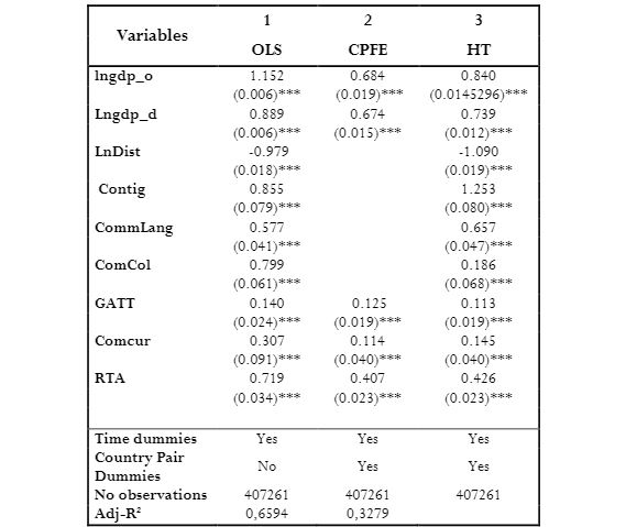
This research has been divided in four steps: the OLS model that has included the GDP of origin and

destination in logarithms, the distance in logarithms, and the following dummies: contiguity (1 if they are contiguous), common language (1 if they speak same language), common colonizer (1 if yes), if origin and destination are GATT (General Agreement on Tariffs and Trade) members (1 if yes), common currency (1 if yes), and if both countries have RTAS signed (1 if yes). In this model, temporary dummies have been included.

The second model is the CPFE model for controlling for unobserved heterogeneity across country pairs. The third model is the (HT) regression, with the same variables as before. It is going to use this model to compare between real and predicted trade. The fourth model is the PPML in order to eliminate the bias for heteroscedasticity and treat the presence observations with zero exports. The following table shows the results for the first three models and the fourth will be presented in a separated table.

Table 1
Main Results of different estimations: Ordinary Least Squares (OLS), Country Pair Fixed Effects (CPFE) and Hausman Taylor (HT).

Elaboration: Author

First is time for analyzing the column (1), which is OLS model. As it has been working with logarithms, the coefficients represent the elasticities of these variables. The estimated coefficients are as expected. Thus, for 1% that the GDP of the exporter grows, the exports grow in 1.15%. Same for GDP in destination (0.88%) and for Distance if exporter is 1% more far exports decrease in 0.97%. For the rest of the variables the explanation is quite similar: if countries are contiguous, or have common language, or have common colonizer, or both are GATT members, or both have RTAs signed, the corresponding value for the dummy is 1. It is important to recall that for dummies, it must calculate the antilogarithm in order to determine the real affectation to the endogenous variable.

Thus, when both countries are contiguous, exports increase in 135%.3 When both have common language, exports increase in 78%; when both countries have common colonizer in 122%; when both are GATT members in 15%; if both have common currency, rise in 35%; and if both have RTAs signed, the exports increase in 105%. All the variables are statistically significant in a 1% confidence level.

The second column shows the main results of the fixed effects regression. The process has finally removed the distance, contiguity, common language, and common colonizer, due to invariability of these among time. Thus, the software has removed because of colinearity. The interpretations of the variables are the same as OLS. The third column shows the Hausman Taylor model with its main results. The interpretations of the coefficients are the same as OLS model. When analyzing significance, same as the other models: all variables are statistically significant with a 1% confidence level. As HT combines fixed and random effects, it has considered the results of the estimation to predict the trade and compare with the real one.

Figure 13 shows a comparison between the real and the predicted (with the Hausman Taylor model) exports between Ecuador and its ten best partners, for each five years, being the 1975 the reference and starting period.

Figure 7
Comparison between Real and Predicted Exports with the Hausman Taylor Model, between Ecuador and its top ten trading partners.

Note: The volumes of exports are in logarithms.

In this section it can highlight three important points. On the one hand, it is seems that since 1985 the opening to foreign trade (with most countries) began to emerge: after the return to democracy at the end of 1979, added to the oil boom of the decade of 70's. These events led the country to a path towards globalization. The second important point that can be observed is that with some countries, for the year 2000, exports decreased due to the financial crisis suffered by the country that led to a ‘banking holiday’ and the chronic consequence of dollarization as a stabilization mechanism and that from there could be a great ally for the Ecuadorian economy to remain solid and stable, but that having no monetary policy would also influence Ecuador's international trade. For this reason, in subsequent paragraphs an additional model will be included that explains its incidence (and whether it has been positive or negative) in the Ecuadorian international trade.

Moreover, it can be seen that since 2005 the volume real exports grow compared to the predicted ones was really significant. This has been largely because it started in 2007; there were export promotion programs, credits and other actions that always led to a position towards globalization. Hence, in most trading partners, Ecuador has had a position towards globalization and trade liberalization, despite the few trade agreements it has and the export potential that may be even greater. Moreover, it has the emergence of new partners as China and Vietnam, that although for a good time real exports were lower than predicted, from 2005 they began to surpass in large quantities, demonstrating the great trade openness that Ecuador has had with these partners, but especially who have become big emerging partners.

But on the other hand are cases as Colombia and Peru, which apparently its closeness in distance, common language, good relations among the history, was supposed to face a permanent surplus between real and predicted. But the reality says that almost all the time the real trade was lower than the predicted. This would probably mean that these three countries have really good trade openness, RTAs, good commercial relations but the predictions say that it was supposed to be even better and could be a call to improve this scenario.

In Figure 14, we show a comparison between the real and the predicted (with the Hausman Taylor model) imports between Ecuador and its ten best partners, for each five years, being the 1975 the reference and starting period. It is important to remember that for this exercise, the main origins of Ecuadorian imports were taken as reference. On the other hand, as the coefficients of the model are the same in general and the data obtained is from exports, it was applied to exports from the country of origin to Ecuador (which are Ecuadorian imports from that origin). Moreover, fixed effect variables do not vary, e.g. is the same distance from Ecuador to Spain, that from Spain to Ecuador, or have common language Colombia and Ecuador either in export or import. For temporary dummies, the values are constant as well.

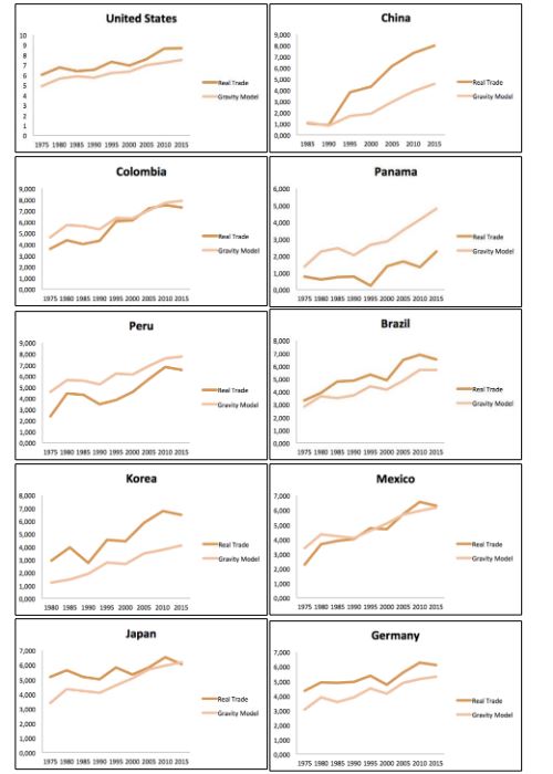Figure 8
Comparison between Real and Predicted Imports with the Hausman Taylor Model, between Ecuador and its top ten trading partners.
Note: The volumes of exports are in logarithms.

The first country in the top ten is the United States and China. As it can be noticed, since 1970 it has been a great partner for Ecuador and real trade has always been higher than predicted with Hausman Taylor. Second goes China, and the scenario is quite similar than the US. China has become a really important partner for Ecuador, even because until 1990 the real and the predicted were practically the same amount and was quite low. From there, the real growth on the predicted has grown very significantly.

On the other hand are cases as Colombia, Panama and Peru, which are the third, fourth and fifth in the top ten according to the last decade. A priori, as they are neighbors (Colombia and Peru) or really close to Ecuador (Panama), the real trade seems to be higher in comparison with the predicted with Gravity Model. Although they amounted big quantities of sales to Ecuador during the last decade, the real level of imports is still lower than predicted. For this reason it is that, at least with Colombia and Peru, an estimate will be presented to measure the effect of being a member of the Andean Community in Ecuadorian international trade.

Just to summarize, it can be noted that with most of the top ten origins of Ecuadorian imports, real amount has been higher than forecast and this shows the trade openness that the country has had. It must also highlight the cases as Colombia, Peru and Panama, which despite being close and even contiguous, and that the quantities imported were very high, trade should be even higher than it already is.

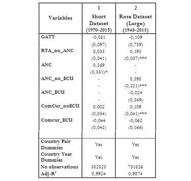
Now let’s move to the final model. Table 2 shows the PPML. It is necessary to recall that this model corrects the problem of heterokedasticity and the loss of information due to the existence of zero trade flows. It is also important to clarify that for the estimation of this model, (Glick & Rose, 2016) suggest that as the number of observations in the database to be used increases, the coefficients for currency union are higher and more significant. Thus, it has made the estimation with the same dataset used for the explained variables and the results have not been significant.

Therefore, it has decided to use the Rose dataset (1948-2013), which has many more observations4, so that the results are more accurate. Likewise, it is relevant to recall that the aim of this model also involves analyzing the effect on Ecuadorian exports that Dollarization has had and the fact of being a member of the Andean Community. Thus, table 2 shows the results of the PPML estimator.

Table 2
Poisson Pseudo-Maximum Likelihood Estimator: Structural Gravity Estimation (country-pair and country-year fixed effects).

Note: ANC= Andean Nations Community; ECU= Ecuador

Table 2 includes two columns. The first column includes the results of the short base and the second includes the results of the dataset from Rose. Let’s start talking about the first column, the ‘short dataset’ that it used for this research for the rest of the models. As it can be noticed, the dummy for ANC is statistically significant only at 10% and if it wanted to be more precise and use a more adjusted level of significance (5%), the variable would not to be significant anymore. It does not talk about the coefficients and their effects because all the variables are not statistically significant. Thus, this is the main reason of having computed a new estimation with a larger dataset as Rose suggests.

According to second column of Table 2, Speaking specifically about the variables, it can say that if both countries are members of the GATT, the variable is not significant at 10 %, meaning that being a GATT member and trading with another member does not contribute to exports, paradoxically with the results of the previous models. On the other hand, if all the RTA minus the ANC were taken into account, exports increase by 21.53% and the variable is statistically significant by 1%.

But the interesting thing about these results comes next. The variable ‘ANC_ECU’ measures the impact of the ANC (with Ecuador included) with its respective exports and ‘ANC_noECU’ excludes Ecuador from that estimate. Under this brief clarification, it can realize that the ANC when it is excluded has a positive contribution of exports of 81.8% and the coefficient is statistically significant at 1%. On the other hand, when it includes Ecuador is not statistically significant. This allows us to infer that being part of the Andean Community does not contribute to the growth of Ecuador's exports.

Another important point of the estimation is with the following variables to measure the effect of dollarization on Ecuadorian exports. The variable 'comcur_noECU' excludes Ecuador from having common currency (in this case the dollar) and 'comcur_ECU' includes it. It can realize that if it excludes Ecuador, exports grow by 11.51% and the variable is statistically significant at 1%. But if it includes Ecuador coefficient is not significant or 10%. This can be corroborated with the reality of the country. Given that Ecuador does not have monetary policy and cannot print banknotes, when either Colombia or Peru has deficits in their trade balance they depreciate their currency and their products fall in price, becoming more competitive with Ecuadorian prices, encouraging exports and decreasing Ecuadorian. Therefore, dollarization may have brought internal economic stability, but in terms of exports it has not contributed to improve.

V. CONCLUSIONS

In this research, it firstly analyzed the main features of the Ecuadorian trade policy. In reference of exports, they grew by 14% in 2015 in comparison with 2014. Moreover, the ten main destinations of international sales are United States, Chile, Vietnam, Peru, Colombia, Russia, Panama, China, Spain and Germany. In reference with imports, they grew by 22% compared to 2014; main origins of imports were China, the European Union, the United States, Colombia, Brazil, Peru, South Korea, Mexico, Panama, Japan, and Germany.

Now let’s talk about the results of the estimations of the gravity model. It has noticed that for all estimations (OLS, CPFE, HT), the variables were statistically significant at 1%. Using HT estimation, it showed a comparison between the real and the predicted trade (exports and imports) between Ecuador and its top ten partners (destinations and origins. It found that with most trading partners, Ecuador has had a position towards globalization and trade liberalization, despite the few trade agreements it has. The strangest point was the case with Colombia and Peru that, despite being neighbors and being members of the Andean Community, the predicted trade was greater than the real for almost the entire period of the research.

Finally, since the actual trade with the members of the Andean Community has been lower than predicted, the PPML model was included to measure the impact of this agreement with Ecuador and without it, and the impact of having a currency union. The results obtained reveal that trade among members of the bloc is positive and significant without Ecuador, but not significant when this country is included. Moreover, the results obtained show that having a common currency without Ecuador has a positive impact on trade, and again not for Ecuador. This allows us to conclude that being part of this block and having dollarized the economy has not significantly benefited Ecuador's trade, which is a disturbing result, and this would be part of a future research.

References

Anderson, J. E., & Wincoop, E. v. (2003). Gravity with gravitas: a solution to the border puzzle. American economic review, 93 (1), 170-192.

Behar, A., & Nelson, B. D. (2014). Trade Flows, Multilateral Resistance, and Firm Heterogeneity. Review of Economics and Statistics, 96(3), 538-549.

Cámara de Comercio de Quito. (2018). Boletín Comercio Exterior. Boletín Comercio Exterior, 1-7.

Chaney, T. (2018). The gravity equation in international trade: An explanation. Journal of Political Economy, 126(1), 150-177.

Clark, T. S., & Linzer, D. A. (2015). Should I Use Fixed or Random Effects? Political Science Research and Methods, 3 (2), 399-408.

Glick, R., & Rose, A. K. (2016). Currency unions and trade: A post-EMU reassessment. ELSEVIER, 79- 91.

Global Edge Portal of the State University of Michigan. (2017). globalEDGE. Retrieved from Your Source for Global Business Knowledge: https://globaledge.msu.edu/countries/ecuador/tradestats

Gómez-Herrera, E. (2012). Comparing alternative methods to estimate gravity models of bilateral trade. Empirical Economics, 44(3), 1087-1111.

Greene, W. H. (2017). Econometric Analysis. New York : Pearson.

Henao-Rodríguez, C., Lis-Gutiérrez, J.-P., Viloria, A., & Ariza, J. (2016). Application of a gravity model in the evaluation of the determinants of intraindustrial trade in Colombia. International Journal of Control Theory and Applications, 9 (44), 1-6.

Kimura, F., & Lee, H.-H. (2006). The Gravity Equation in International Trade in services. Review of World Economics, 142 (1), 92-121.

Ministerio de Comercio Exterior e Inversiones del Ecuador. (2014). El Acuerdo Comercial Ecuador - Unión Europea. Revista del Ministerio de Comercio Exterior, 1-24.

Ministerio de Comercio Exterior e Inversiones del Ecuador. (2015). Boletín Mensual de Comercio Exterior. Dirección de Estudios Económicos y Comerciales, 1-28.

Van Bergeijk, P. A., & Brakman, S. (2010). The gravity model in international trade: Advances and applications. New York: Cambridge University Press.

Wooldridge, J. (2015). Introductory econometrics: A modern approach (4th ed.). Michigan, Ohio, USA: Nelson Education, Ltd.

Wooldridge, J. M. (2002). Econometric Analysis of Cross Section and Panel Data (Vol. 58). Cambridge.

APPENDIX

Table A1
List of Countries

Elaboration: Author

Notes