I. Introduction

The presumption that the expectations of economic agents should be described as derived from the model proposed by the analyst has been a centerpiece of macroeconomic analysis for several decades already. However, model- consistency, and rational expectations itself, are ambiguous, ill- defined concepts, the practical implementation of which raises issues of logical coherence (see, e.g., Heymann and Pascuini, 2017).

In his seminal paper, Muth (1961) formulates the rational expectations hypothesis as: “the expectations of firms (or more generally, the subjective probability distribution of outcomes) tend to be distributed, for the same information set, about the prediction of the theory (or the ‘objective’ probability distribution of outcomes).” It can be noted that both meanings are not identical: the prediction of the theory is contingent on the varying state of knowledge or professional opinion, which cannot claim perfect accordance with the facts. We are interested in the implications of that distinction.

In turn, Sargent (2008) states that: “a rational expectations equilibrium is a fixed point of this mapping (from perceived law of motion to actual law of motion)... From a practical perspective, an important property of a rational expectations model is that it imposes a communism of models and expectations. If we define a model as a probability distribution over a sequence of outcomes..., a rational expectations equilibrium asserts that the same model is shared by (1) all of the agents within the model, (2) the econometrician estimating the model, and (3) nature, also known as the data generating mechanism.”

However, the equivalence between the three perspectives can hardly be sustained. In the (2)–(3) dimension, if the economist presumes that her model strictly corresponds to the DGP, she ignores the observable fact that her theories and models have changed over time, while her current engagement in research indicates a recognition that her knowledge has not converged to an accurate representation of the phenomena of interest, and that there remains ample room for revisions, improvements and refinements. Therefore, the laws of motion described by (2) and (3) do not coincide, as clearly acknowledged in the active work that has been ongoing about model selection and “countefactual equivalence” (e.g., Beraja, 2018, Canova, 2009, Giannone et al. 2018), specification searches (Ahumada, 2018), and model uncertainty (Hansen, 2017; Hansen and Sargent, 2000, 2018).

On the (1)–(3) link, the recognition that economic actors are involved in learning about their environments has led to representations of “agents as econometricians”, or users of heurístic procedures tio make forecasts (Sargent 1993, 2001, Evans and Honkapohja, 2001, Barberis et al., 2016, Hommes, 2017). In the event the assumption that agents act as if their expectations were derived from the true DGP is maintained, the existence of gaps in the (2)–(3) connection implies that the analyst should consequently recognize the inferiority of her model compared with the (tacit) knowledge of agents, incorporated in their forecast- making schemes. Thus, the modeler who affirms the (1)–(3) equivalence should not identify the probability distribution of future events perceived by agents with that drawn from her imperfect construct.

Our focus here is on the (1)–(2) connection, that is, on the notion that the expectations of agents are compatible with those generated by the “relevant economic theory”, taking as given that neither of them approximate the actual laws of motion of the variables of interest. Now, the relevant theory is a dated object: the variability of economic analysis makes model- consistency an imprecise concept.

Standard practice in Macroeconomics uses a quite special form of model- consistency (MC-a), in which the expectations of agents formed at all times are represented as derived from the model currently proposed by the analyst. But that assigns to agents in the past more knowledge than the economist then possessed (since, when proposing the latest research product, the analyst sees it as an advancement relative to previous vintages).

Alternatively, model- consistency can be conceived as a correspondence of the expectations- generating scheme used by agents with the model that the analyst (or the theoretical dynasty to which the present modeler belongs) considered the appropriate tool to understand and forecast the matters of interest when the expectations were being formed. This second version (M-Cb) would correspond to the intuitive argument that the economically pertinent beliefs and behaviors at a certain moment are influenced by the professional views current at the time, and would depict agents as learning (and erring) in parallel with the “representative economist” of the current analyst’s lineage. Model-consistency would then contemplate (in an extreme form) the potential repercussions of economic research on actual behavior, and would allow for non-random mistakes in expectations (judged from the point of view of the now- incumbent model) which were based at their time on now past analytical schemes.¹ As far as we know, the notion of M-Cb, which makes the specification of expectations-relevant models evolve with the changes in accepted macro analysis has not been investigated as such in the literature.

The aim of the paper is to explore the application of the alternative definitions of model-consistency , that is, we concentrate on the (1)–(2) axis, where the forecasts of the agents are seen in connection with those derived by (variously defined) analytical predictions (which, in turn depend on hypotheses on expectations embedded in the corresponding models). In particular, we want to study the practical implementation of the M-Cb notion in a concrete instance. For the purpose of the exercise, we abstain from formulating a specific model; rather, we use two simple existing examples of different generations, both members of a family with wide circulation, and built to be applied to the US. The older one (M1, of a type current starting in the 1970´s) stresses the response of output to unanticipated changes in the money supply (à la Bohara, 1991, related to Barro, 1978, Mishkin, 1982a), while M2 is more recent (mid 2000’s) small New Keynesian model where the policy instrument is the interest rate and monopolistic competitors are subject to Calvo-type (1983) restrictions on price movements (see Cho and Moreno, 2006). In both models, agents must form anticipations to determine their behavior; in each case, the original M1 or M2 models represented expectations as in M-Ca, assuming that that those expectations had been based in the past on the current model, and would remain to be based on it in the future.

In the exercise, we take as given that the later model, M2, was meant to specify the relevant structure for all times and we consider its working in conjunction with expectations generated either by the same model (M2), or by that of the previous generation, M1. We then take the alternative specification to the US data (different 20-year rolling windows between 1959 and 2015), and check whether the alternative expectational schemes make a difference on the estimates (the specifics of the procedures are discussed in the following section). In so doing, we are stepping into the (1)-–(3), agent-DGP dimension. The objective of the exercise is thus simply to try out the implementation of the versions of model-consistency.

This paper is organized as follows. Section II summarizes the procedure used to evaluate model-consistency. Section III describes the macroeconomic models, M1 and M2, on which the exercises will be basedM2 and M1 models. Section IV develops Wald tests for the restrictions associated with the different versions of model-consistency Section V presents the empirical results. Section VI concludes.

II. Procedural issues

Model-consistency tests (of the M-Ca) type were performed some decades ago on M1 models, in different ways. Mishkin (1982a,1982b), for instance, did not estimate a structural form; rather, he focused on checking whether some parameters of the reduced form were zero, as implied by the theory. Concerning this kind of Wald tests, Gregory and Veall (1987) pointed out that they are quite sensitive in small samples to the way in which the non-linear restrictions are parametrized. Alternative tests were proposed by Hoffman and Schmidt (1981) and Godfrey and Veall (1985a,1985b). Hatcher and Minford (2016) present an alternative strategy for testing M-Ca: the “indirect inference procedures”. The suggestion there is to compare the VAR parameters drawn from the data and the mean VAR coefficients estimated from bootstrapped samples from the full macro model, after imposing the restrictions on parameters implied by the theory. In our case, the unconstrained model M2 can be estimated without difficulty, and then Wald tests are then preferred to alternatives such as Lagrange multipliers and likelihood ratio tests. In this regard, it is known that non-linear restrictions on structural parameters may imply complicated (or non-convergent) iteration processes; thus the convenience of using the unrestricted model, as allowed by the approach we follow here. For a broader discussion, see, for example, Hatcher and Minford (2016), Le et al. (2011), Liu and Minford (2014).

The exercises that follow use non-linear Wald tests derived from estimations with the generalized method of moments (GMM). For the M-Ca(M2, M2) case, the procedure can be summarized as follows. For each time window, the first step is to estimate a data-driven forecasting scheme through a vector autoregressive (VAR) model, using the variables that appear in the M2 model (aggregate output, inflation and the policy interest rate). The predictions generated through the corresponding reduced form equations are fed into the structural M2 model, and the structural parameters are then estimated (here, using an instrumental variables approach to deal with endogeneity issues). The equations of the corresponding reduced form can then be obtained. As for the exercise that applies the M-Cb(M2,M1) notion, the first stage is as before, because it is carried out without reference to theories and, since M2 is maintained as the assumed structure, the second leg (estimating the model’s structural parameters with expectations drawn from an unrestricted VAR) is also the same. But, next, model M1 is used to produce expectations in the manner of M-Ca(M1,M1), that is, with the constraints imposed by the specification of the model. Then the corresponding forecasts are used to estimate the structural parameters of M2. In both cases, the final operation is to check whether the parameters of the structural- based set of reduced form equations are significantly different from those of the unrestricted equations found in the first step. If the answer is positive, the hypotheses (either M-Ca(M2,M2) and/or M-Cb(M2,M1)) are considered to be rejected.

In our application, for most of the time interval under consideration, neither M-Ca(M2,M2) nor M-Cb(M2,M1) is rejected. The tests seem to lack power to discriminate between roughly similar models (and possibly between them and other alternatives) as forecast-generators, in a period of relative tranquility in the economy in question. However, when we consider more recent sample periods, with information after the eruption of the crisis of the late 2000’s, the parameters of the estimated model (particularly the output gap equation) become unstable, pointing to the existence of problems in the performance of the models.

III. The basic M2 and M1 models

III.1 M2: a small New Keynesian Model

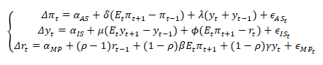
The New Keynesian Model (NKM) proposed by Cho and Moreno (2004, 2006) consists of a small (three- equation) system with three endogenous variables, ${\mathrm{\pi }}_t$, $y_t$ and $r_t$, standing for inflation, the output gap, and the policy nominal interest rate, respectively. Each equation exhibits persistence effects and has forward- looking terms. As usual with small NKM models, the equations represent the aggregate supply schedule (AS), the demand for goods function (IS), and the rule followed by the monetary authorities to determine the interest rate (MP).

The AS curve is a modification of Fuhrer and Moore (1995), where the inflation rate is determined by inflationary expectations, an inertial effect of past price increases and the current and lagged output gaps. Thus:

(1)

where ${∊}_{{\text{AS}}_t}\sim i.i.d.(0,\mathrm{\sigma }\genfrac{}{}{0ex}{}{2}{\text{AS}})$is the aggregate supply structural shock. ${\text{E}}_t$ is the expected value operator, conditional on available information at time $t$.

The IS equation is a typical goods-demand function with habit-persistence effects as in Fuhrer (2000), where the output gap results from the expected future level of aggregate production, lagged output and the ex-ante real interest rate:

(2)

where ${\in }_{{\text{IS}}_t}\sim i.i.d.(0,\mathrm{\sigma }\genfrac{}{}{0ex}{}{2}{\text{IS}})$ is the aggregate supply structural shock.

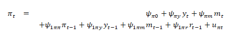
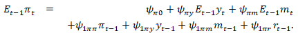
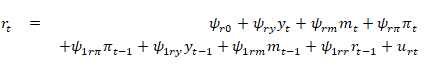
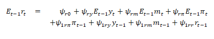
Finally, the monetary policy equation, MP, models the policy nominal interest rate through a reaction function conditional on expected inflation and the output gap, with a smoothing autoregressive term (see Clarida, Galí and Gertler (2000)):

(3)

where is the monet

where ${\text{ϵ}}_{\text{MP}}~i.i.d.(0,\sigma \genfrac{}{}{0ex}{}{2\hfill }{\text{MP}})$ is the monetary policy structural shock.

The equations can be summarized as$$\begin{gathered} \left[\begin{array}{ccc}\mathrm{1}& -\lambda & 0\\ \mathrm{0}& 1& \mathit{\text{ϕ}}\\ \mathrm{0}& -(1-\rho )\gamma & 1\end{array}\right]\left[\begin{array}{c}{\pi }_t\\ y_t\\ r_t\end{array}\right]= \\ \left[\begin{array}{c}{\alpha }_{\text{AS}}\\ {\alpha }_{\text{IS}}\\ {\alpha }_{\text{MP}}\end{array}\right]+\left[\begin{array}{ccc}\delta & 0& 0\\ \mathit{\text{ϕ}}& \mu & 0\\ (1-\rho )\beta & 0& 0\end{array}\right]{\text{Ε}}_t\left[\begin{array}{c}{\pi }_{t+1}\\ y_{t+1}\\ r_{t+1}\end{array}\right]+ \\ \left[\begin{array}{ccc}1-\delta & \lambda & 0\\ 0& 1-\mu & 0\\ 0& 0& 0\end{array}\right]\left[\begin{array}{c}{\pi }_{t-1}\\ y_{t-1}\\ r_{t-1}\end{array}\right]+\left[\begin{array}{c}{\text{ϵ}}_{{\text{ΑS}}_t}\\ {\text{ϵ}}_{{\text{IS}}_t}\\ {\text{ϵ}}_{{\text{MP}}_t}\end{array}\right]· \end{gathered}$$

In compact matrix notation the model can be expressed as:

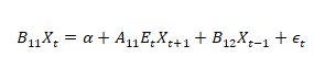(4)

where ${\mathit{\text{X}}}_t=\left({\pi }_t,y_t,r_t\right)\mathit{\text{'}}$ is the vector of endogenous variables,${\mathit{\text{Β}}}_{11}=\left[\begin{array}{ccc}1& -\lambda & 0\\ 0& 1& \mathit{\text{ϕ}}\\ 0& -(1-\rho )\gamma & 1\end{array}\right]$ , ${\text{Α}}_{11}=\left[\begin{array}{ccc}\delta & 0& 0\\ \mathit{\text{ϕ}}& \mu & 0\\ (1-\rho )\beta & 0& 0\end{array}\right]$ , and ${\text{Β}}_{12}=\left[\begin{array}{ccc}1-\delta & \lambda & 0\\ 0& 1-\mu & 0\\ 0& 0& \rho \end{array}\right]$ are the coefficients matrices of structural parameters, $\alpha$ is the vector of constants, and ${\text{ϵ}}_t\sim (0_3,\text{D})$ is the vector of structural errors with $\mathit{\text{D}}$ a diagonal variance matrix. Define $\eta =\left(\delta ,\lambda ,\text{μ},\mathit{\text{ϕ}},\beta ,\gamma \right)\text{'}$ as the multivalued parameter of interest.

Note that one of the key characteristics of the model is that agents base their decisions on expectations about the future value of the vector ${\mathit{\text{X}}}_t$ , ${\mathit{\text{E}}}_t{\mathit{\text{X}}}_{t+1}$.

III.2 M2-NKM expectations

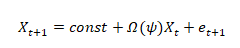
Cho and Moreno (2006, p.1464, eq. (4)) shows that the assumption of no asymmetric information between the economic agents and the monetary policy authority implies a forecasting mechanism of the form

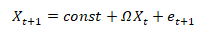(5)

where $e_{t+1}=\mathit{\text{Γ}}{\mathit{\text{ϵ}}}_{t+1}$ and $\mathit{\Omega }$ and $\mathit{\text{Γ}}$ are $3\times 3$ matrices.

Define $\omega =vec\left(\mathit{\Omega }\right)=\left({\omega }_{\pi \pi },{\omega }_{\pi y},{\omega }_{\pi r},{\omega }_{y\pi },{\omega }_{yy},{\omega }_{yr},{\omega }_{r\pi },{\omega }_{ry},{\omega }_{rr}\right)$ as the autoregressive parameters in (5).

III.3 M1 model and expectations

In the 1970’s and early 1980’s, a highly prominent family of models, originated from works like Lucas (1972), Sargent and Wallace (1976), Barro (1977), represented the determination of the aggregate supply of goods as a function of monetary (or price) surprises, while macro policy was assumed to operate through changes in the magnitude of the money supply; in addition, the models applied the standard M-Ca presumption for expectations. Given their influence in academic environments and in public discourse during a substantial lapse of time, those theories stand up as candidates for having been used for expectations- formation during at least part of the period of interest.

In order to define a concrete and simple instance (M1) of such models, we use a streamlined version based on Barro (1978), Mishkin (1982a, 1982b) and Bohara (1991). A formal property of the model is that it can be solved recursively for a structural vector autoregression identified through a Cholesky decomposition, with a hierarchy of effects: first the, monetary aggregate is forecasted, allowing to determine aggregate output, next inflation and, finally, interest rates.

The specification of the model starts with a reaction function of the central bank which, as in Bohara (op. cit.), gives the growth rate of the money supply at time $\textcolor{red}{}t$ given the values at $t-1$ of cyclical output and the interest rate, and its own lagged value. It can be noted that the equation does not allow for a direct response of monetary policy to the inflation rate. In this, we follow the assumptions made in the previously cited papers, which we take as embodying accepted views at their times: we are not interested in building a model per se, but in identifying what could be seen as a “representative” member of the models of the earlier generation. Then:

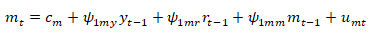(6)

Now, the aggregate supply equation expresses the deviation from trend of total output as a function of unanticipated money supply, anticipated money (to allow for possible non- neutralities) and an autoregressive term:

(7)

where ${\psi }_{ym1}$ reflects the non-neutrality of money (as highlighted in Mishkin, op. cit., and subsequent works) and ${\psi }_{ym2}$ the effect of unexpected shocks on output.

Using the two previous equations, the model-based expectation of the cyclical component of output can be obtained as:

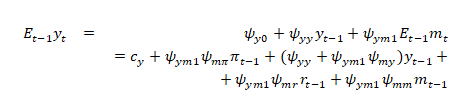(8)

The inflation rate is derived, as was common at the time, from a simple money demand function in the spirit of the quantity theory. The equation we postulate is:

(9)

and the corresponding inflation expectations determined from the model are:

(10)

The system up to this point allows to define anticipations for the money supply, cyclical output and prices. There is here (as in the references quoted above) no equation determining the interest rate. But that variable is needed when combining the later- vintage M2 model with M1 expectations. For that purpose, we write an unrestricted equation where the interest rate is expressed as depending on the other three variables (and their lags):

(11)

Then, the interest rate forecasts implied by the model would be:

(12)

It follows that the expectations mechanism implementing version model- consistency of the form M-Ca(M1,M1) can be expressed as a function of the $\psi$ parameters above

(13)

where $\mathrm{\Omega }$ depends on the $\psi$ parameters and ${\mathit{\text{X}}}_t$ is the vector of the three endogenous variables used for M2, $\left({\pi }_t,y_t,r_t\right)$.

III.4 Model-consistency as parameter restrictions

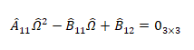
The model-consistency of the M-Ca(M2,M2) and M-Cb(M2,M1) types implies a simultaneous solution of eqs. (4) and either (5) or (13), respectively. Cho and Moreno (2004,2006) solves a macroeconomic model with M-Ca(M2,M2) by imposing the simultaneous solution of the structural model (perceived law of motion) and the VAR(1) model (understood as the actual law of motion), which implies the restrictions:

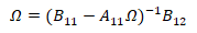(14)

This condition can be written as a quadratic matrix equation:

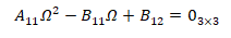(15)

Note that this implies nine nonlinear restrictions involving both $\eta$ and $\omega$, which can be summarized by:

where $\theta =({\eta }^{\text{'}},{\omega }^{\text{'}})\text{'}$, $\eta$ are the structural parameters and $\omega$ the VAR(1) reduced-form parameters, as defined above.

Our model-consistency tests ask about the validity of this restriction using Wald specification tests of (16).

IV. Wald statistics for model-consistency

The classical framework allows for three different types of specification tests. First, we could implement a likelihood ratio statistic that contrasts the values of the objective function corresponding to the unrestricted model with the model incorporating the restrictions coming from (16). A second option would be to use a Lagrange multiplier statistic based on the score functions derived from the objective functions pertaining only to the restricted model. Or, one could perform a Wald statistic computing the asymptotic distribution of $a\left(\theta \right)$ using only the unrestricted model.

The first two procedures involve the estimation of the restricted model, implying the simultaneous solution of the economic model and the law of motion (given by the VAR representation), subject to eq. (16). Cho and Moreno (2004, 2006) propose a simultaneous estimation procedure of the above model using a maximum likelihood estimator. However, the non-linearity restrictions on the structural parameters could potentially involve multiple stationary or complex valued solutions, or even no solutions at all (i.e., no convergence of the iteration process). Accordingly, for testing purposes in this case, there would be a strong preference for using the unrestricted model and tests based on Wald statistics.² The Appendix reviews the asymptotic properties of Wald tests for time-series models under the GMM framework.

In the exercises carried out in this paper, the implementation of the Wald test is done through the following steps. First, we run the reduced form VAR(1) models (5) or (13), that is, without imposing any restriction.

Then we consider the structural model M2-NKM eq. (4), which can be written as:

(17)

The next stage is to replace ${\text{E}}_t{\text{X}}_{t+1}$ by ${\hat{\text{X}}}_{t+1}$ resulting from the VAR models estimated in the first step, using either the results of (5) or (13) according to whether one is considering the case of M-Ca(M2, M2) or that of M-Cb(M2, M1). It can be noted that it is not possible to obtain consistent least-squares estimators of the structural parameters as ${\hat{\text{X}}}_{t+1}$ contains ${\mathit{\text{X}}}_t$. This is solved by running instrumental variables (IV) estimators where the endogenous variables are instrumented by ${\widehat{\mathit{\text{X}}}}_{t-1}$ . Consistency is guaranteed by the assumptions on $\mathit{∊}$.

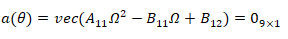
Given the parameters of the VAR reduced form, represented by the matrix $\hat{\mathrm{\Omega }}$, and using the corresponding expected values in equations (17) the structural parameters in those equations can be estimated, giving the three matrices $\left({\hat{\text{A}}}_{11},{\hat{\text{B}}}_{11},{\hat{\text{B}}}_{12}\right)$. Then, the nine non-linear restrictions can be written as:

(18)

Consider now those parameter restrictions expressed in extensive form as a $9\times 1$ vector function, $a\left(\theta \right)$ . Define $\theta ={\left(\delta ,\lambda ,\mathit{\mu ,\varphi },\rho ,\beta ,\gamma ,{\omega }^{\prime }\right)}^{\prime }$ as the $p=7+9$ parameters and the equality $a\left(\theta \right)=0_{9\times 1}$ given by

(20)

Note that $a\left(\eta ,\omega \right)=vec({\text{Α}}_{11}\left(\eta \right){\mathit{\Omega }}^2\left(\omega \right)-{\text{Β}}_{11}\left(\eta \right)\mathit{\Omega }\left(\omega \right)+{\text{Β}}_{12}\left(\eta \right))$ then ${\partial }_{\eta j}a\left(\eta ,\omega \right)=vec({\text{Α}}_{11}\left(\eta \right){\mathrm{\Omega }}^2\left(\omega \right)-{\partial }_{\eta j}{\text{Β}}_{11}\left(\eta \right)\mathrm{\Omega }\left(\omega \right)+{\partial }_{\eta j}{\text{Β}}_{12}\left(\eta \right))$ and ${\partial }_{\omega \kappa }a\left(\eta ,\omega \right)=vec(2{\text{Α}}_{11}\left(\eta \right)\mathrm{\Omega }\left(\omega \right){\partial }_{\omega \kappa }\mathrm{\Omega }\left(\omega \right)-{\text{Β}}_{11}\left(\eta \right){\partial }_{\omega \kappa }\mathrm{\Omega }\left(\omega \right)))$ . The variance- covariance matrix to be used to apply the Wald statistics can be calculated in the way shown in the Appendix.

V. Results of the Wald tests

Table 1

Wald test statistics

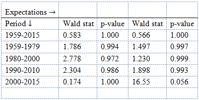
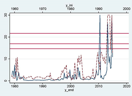
We first report Wald test results in Table 1 for the full sample, 1959-2015, then for several subsamples: 1959-1979, covering two decades before the Volcker era; 1980-2000, which happens to be the period on which Cho and Moreno (2004,2006), the M2 model, was originally estimated, and finally the latest period in the sample, 2000-2015, which includes observations during and after the recent latest financial crisis in the US. The sub-interval 1990-2010 is also considered, to see whether a change in behavior appears in this period. The tests are computed using either $\left({\pi }_t,t_y,r_t\right)$ or $\left({\pi }_t,y_t,r_t,m_t\right)$ to generate forecasts for the tests of M-Ca(M2-M2) and M-Cb(M2-M1), respectively. Figure 1 reports the results of rolling-windows exercises with successive 20-year (80 quarters) samples, so that the estimates cover periods from 1959-1979 to 1995-2015.

For the periods before the year 2000, the tests do not reject either of the model- consistent schemes: thus, they cannot make a sharp selection between alternative specifications of the expectations mechanisms, even though the policy regime changed substantially over the sample periods. The differentiation between the expectational alternatives appears more clearly for more recent periods after 2000, when there is a clear rejection of the anticipations based on the older- generation model, M-Cb(M2-M1), while M-Ca(M2-M2) cannot be rejected. With a closer look, using rolling-window estimates, the performance of the M2 model with M2- compatible expectations also becomes more problematic when observations pertaining to the financial crisis and its aftermath are included. Figure 1 reports the results of rolling-windows exercises with successive 20-year (80 quarters) samples, so that the estimates cover periods from 1959-1979 to 1995-2015. While no rejections are found before 2000, the Wald statistics rejects in several cases for samples that include post-2010 observations, pointing at problems in the performance of the models, and their associated model- consistent expectational schemes, in settings marked by macroeconomic crises.

Figure 1

Wald test statistics for 20-years rolling-windows, 1959-1979 to 1995-2015

Solid line: forecasts using $\left({\pi }_t,y_t,r_t\right)$. Dashed line: forecasts using$\left({\pi }_t,y_t,r_t,m_t\right)$ . Horizontal lines are the 1%, 5% and 10% critical values for a ${\chi }_9^2$ . Wald statistics are capped at a maximum value of 30. For the M-Ca(M2,M2) tests and the sub-samples 1990q3:2010q3 and 1994q4:2014q4 the Wald values are capped. For the M-Cb(M2,M1) tests the sub-samples ending in 2013:q2, 2013:q3, 2013:q4, 2014:q1 and 2014:q4 are capped.

Figure 2

Structural parameter estimates 20-years rolling-windows, 1959-1979 to 1995-2015

Notes: Solid line: forecasts using$\left({\pi }_t,y_t,r_t\right)$ . Dashed line: forecasts using $\left({\pi }_t,y_t,r_t,m_t\right)$. In all figures the parameter values below the bottom 1% and above the upper 99% percentiles are capped.

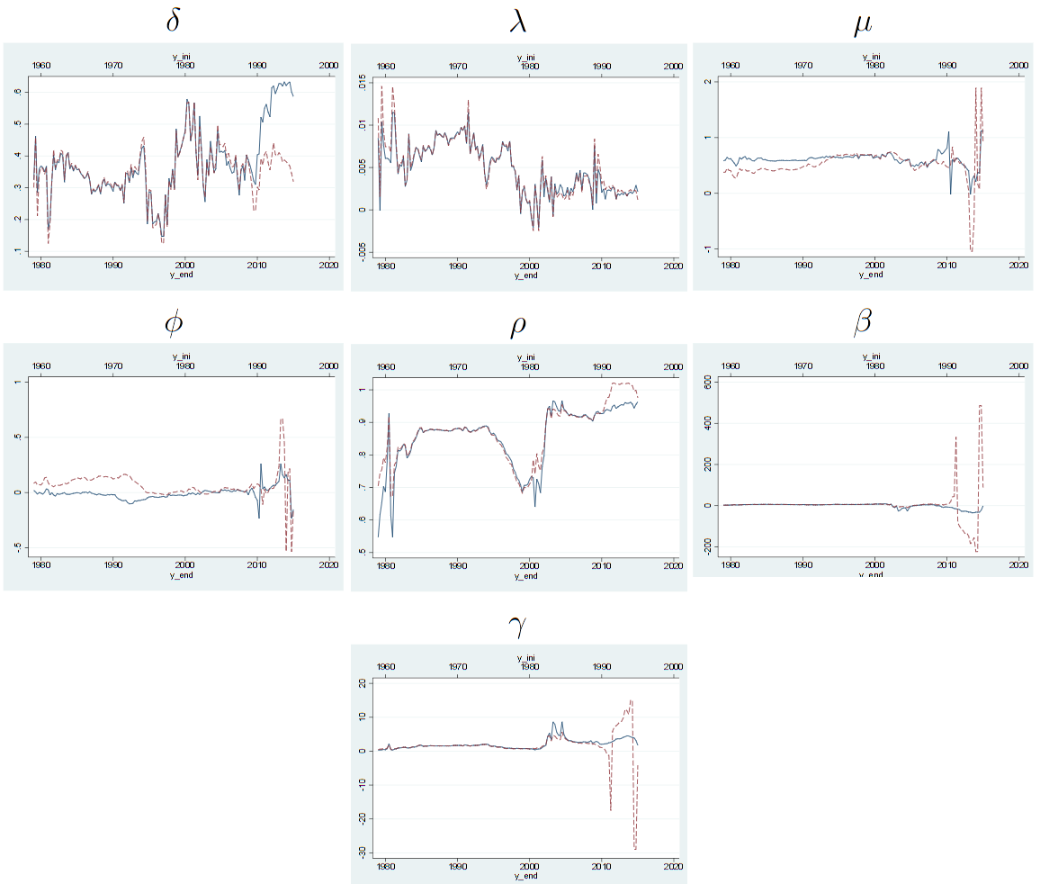
Complementary results can be observed in Figure 7, which reports the estimated parameter values for each sub-sample. While the measured parameters did not show much inter- sample volatility in earlier periods, with values in the range of those found by Cho and Moreno (2006), after 2010 the estimated coefficients present a considerable sensitivity to the specific sample being considered, especially for the parameters of the aggregate demand function (i.e.,$\left(\mu ,\mathit{\text{ϕ}}\right)$ ). Although we do not have a specific hypothesis for this last result we can speculate on the following. From a statistical point of view this indicates that either there was a parameter structural change (very likely because of the magnitude of the crisis) or the structural model changed and resulted in lack of identification of the parameters (and thus they cannot be point estimated with accuracy). From an economic point of view, as suggested by an anonymous referee, this could be an indication of the failure of the aggregate demand.

V. Concluding remarks

Since economic analysis changes over time, model- consistency of expectations is intrinsically a dated concept. Standard practice, which postulates that the expectations of agents are formed for all times (past, present and future) on the basis of the model currently being proposed by the economist, imputes to past decision- makers knowledge and views that the analyst did not hold at the time. If the implicit assumption is that the professional representations of the economy are somehow reflected in actual economic behavior, it would follow as a matter of logic that the schemes used by agents to anticipate expectations have been varying in correspondence with the evolution of influential theories and models. The notion may turn out to be more or less relevant, but in any case it has the feature of allowing to consider a particular learning dynamics, mirroring that of the economists in view (contemporaneous, in this case, rather than long defunct as in Keynes, 1936), and thus to depict expectational mistakes analogous to those of once- incumbent models.

In this paper we have developed an exploratory exercise applying a model-consistency formulation which allows for the drift of expectations- forming tools as theories are modified. The preliminary results obtained suggest that the periods around macroeconomic crises can be particularly interesting periods to focus future research.

A. Appendix

Consider a set of $m$ population moment conditions that will be used to construct GMM estimators (see, e.g., Hansen (1982) and Newey and West (1987)), $\text{E}\left[g\left(z,{\theta }_0\right)\right]$

where $g\left(z,\theta \right)$ is an $m\times 1$ vector of functions of data and parameters, $\textcolor{red}{}z$ is a $k\times 1$ random vector and $\textcolor{red}{}\theta$ is a $p\times 1$ vector of parameters.

When equation above is correct, the sample moments, i.e. $g_{\text{T}}\left(\theta \right)=\frac{1}{\text{T}}{\sum }_{t=1}^{\text{T}}g\left(z_t,\theta \right)$, should be close to zero when evaluated at $\theta ={\theta }_0$.

Let $w_{\mathit{\text{T}}}\left(\theta \right)$ be an $\textcolor{red}{}m\times m$ positive semi-definite matrix. Define the loss function ${\text{Q}}_{\text{T}}\left(\theta \right)=-\frac{1}{2}{g}_{\text{T}}{\left(\theta \right)}^{\text{⊤}}{\text{W}}_{\text{T}}^{-1}\left(\theta \right)g_{\text{T}}\left(\theta \right)$. For asymptotic efficiency and to simplify the analysis we will assume $\underset{\text{T}\to \mathrm{\infty }}{\lim }{\text{W}}_{\text{T}}\left(\theta \right)=\underset{\text{T}\to \mathrm{\infty }}{\lim }\text{V}ar{\left[\sqrt{\text{T}}{g}_{\text{T}}\left(\theta \right)\right]}^{-1}=\text{W}\left(\theta \right)$ and $\text{W}=\text{W}\left({\theta }_0\right)$ (see Hansen (1982) and Newey and McFadden (1994)).

Let ${\nabla }_{\theta }g\left(z,\theta \right)=\partial g\left(z,\theta \right)∕\partial {\theta }^{\top }$ be the $\textcolor{red}{}m\times p$ Jacobian matrix of $g\left(z,\theta \right)$, $\text{G}\left(\theta \right)=\text{E}\left[{\nabla }_{\theta }g\left(z,\theta \right)\right]$ and ${\text{G}}_{\text{T}}\left(\theta \right)=\frac{1}{\text{T}}{\sum }_{t=1}^{\text{T}}{\nabla }_{\theta }g\left(z_t,\theta \right)$. Define the counterpart of the score (pseudo-score) as $\textcolor{red}{}{q}_{\text{T}}\left(\theta \right)=-{\text{G}}_{\text{T}}\left(\theta \right){\text{W}}_{\text{T}}^{-1}\left(\theta \right)g_{\text{T}}\left(\theta \right)$, and $\textcolor{red}{}{q}_{j,\text{T}}\left(\theta \right)$ the $\textcolor{red}{}{p}_j\times 1$ sub-vector. Also, let $\text{Ξ}\left(\theta \right)=\text{G}{\left(\theta \right)}^{\top }{\text{W}}^{-1}\left(\theta \right)\text{G}\left(\theta \right)$, ${\text{Ξ}}_{\text{Τ}}\left(\theta \right)={\text{G}}_{\text{T}}{\left(\theta \right)}^{\top }{\text{W}}_{\text{T}}^{-1}\left(\theta \right){\text{G}}_{\text{T}}\left(\theta \right)$ and $\text{Ξ}=\text{Ξ}\left({\theta }_0\right)$.

Consider a set of $\textcolor{red}{}r$ restrictions given by the vector function $\textcolor{red}{}a\left(\theta \right)$. Define $\textcolor{red}{}\text{Λ}\left(\theta \right)={\nabla }_{\theta }a\left(\theta \right)$ and $\text{Λ}=\text{Λ}\left({\theta }_0\right)$, an $\textcolor{red}{}r\mathit{\times }p$ matrix of rank $\textcolor{red}{}r$.

We are interested in the null hypothesis $\textcolor{red}{}{\text{H}}_0:a\left({\theta }_0\right)$ against $\textcolor{red}{}{\text{H}}_{\text{A}}:a\left({\theta }_0\right)=d/\sqrt{\text{T}}$.

Consider the following assumptions in Newey and West (1987):

[gmm] (i) The data $\textcolor{red}{}{\left\{{\text{Z}}_t\right\}}_{t=1}^{\text{T}}$ are random vectors that are the first T elements of a strictly stationary stochastic process $\textcolor{red}{}{\left\{{\text{Z}}_t\right\}}_{t=1}^{\infty }$ and has a measurable joint density function $\textcolor{red}{}f(z_1,...,z_{\text{T}},\theta )$ with respect to a measure $\textcolor{red}{}{\text{Π}}_{t=1}^{\text{Τ}}v$, where $v$ is a $\textcolor{red}{}\sigma$-finite measure on $\textcolor{red}{}{ℝ}^k$.

(ii) For each $\theta \in \text{Θ}\subset {ℝ}^p$, the elements of $\textcolor{red}{}g\left(z,\theta \right)$ are measurable in $\textcolor{red}{}z$ and $\textcolor{red}{}\int g\left(z,\theta \right)f\left(z,\theta \right)dv=0$.

(iii) The vector $\textcolor{red}{}g\left(z,\theta \right)$ is continuously differentiable on $\textcolor{red}{}\mathit{\text{Θ}}$, almost everywhere $\textcolor{red}{}v$, and $\textcolor{red}{}a\left(\theta \right)$ is continuously differentiable on $\textcolor{red}{}\mathit{\text{Θ}}$. For each positive integer $\textcolor{red}{}n\ge 2$ the joint density $\textcolor{red}{}f(z_1,z_n,\theta )$ is continuous in $\textcolor{red}{}\theta$ almost everywhere $\textcolor{red}{}v\times \upsilon$. Also $\textcolor{red}{}{\theta }_0\in int\left(\text{Θ}\right)$ where $\textcolor{red}{}\mathit{\text{Θ}}$ is compact.

(iv) There exist measurable functions $\textcolor{red}{}{h}_1\left(z\right)$ and $\textcolor{red}{}{h}_2\left(z\right)$, and $\textcolor{red}{}c>1$, such that almost everywhere $\textcolor{red}{}v$, and for all $\theta \in \text{Θ}$ and $\textcolor{red}{}n\ge 2$, $$\begin{gathered} {\mid g\left(z,\theta \right)\mid }^4\le h_1\left(z\right),{\mid \partial g\left(z,\theta \right)∕\partial \theta \mid }^2\le h_1\left(z\right), \\ f\left(z,\theta \right)\le h_2\left(z\right),f\left(z_1,z_n,\theta \right)\le h_2\left(z_1\right)h_2\left(z_n\right), \\ \int {\left[{\gamma }_1\left(z\right)\right]}^c{h}_2\left(z\right)dv<+\infty ,\int h_2\left(z\right)dv<+\infty . \end{gathered}$$

(v) There exist constants $\text{C}$, $\text{ϵ}>0$ such that either, (a) for all $\theta \mathit{\in }\mathit{\text{Θ}}$ , ${\left\{z_t\right\}}_{t=1}^{\mathrm{\infty }}$ is uniform mixing with $\mathit{\text{ϕ}}\left(n\right)\le \mathit{\text{C}}{n}^{-ϵ}$, $\text{ϵ}\ge \max \{2,c/(c-1\left)\right\}$, (b) for all $\theta \in \mathit{\text{Θ}}$, $\textcolor{red}{}{\left\{z_t\right\}}_{t=1}^{\mathrm{\infty }}$ is strong mixing with $a\left(n\right)\le \mathit{\text{C}}{n}^{\mathit{-ϵ}}$ , $\textcolor{red}{}\mathit{\text{ϵ}}\ge \max \{2,c/(c-1\left)\right\}$ .

(vi) For all $\theta \in \mathit{\text{Θ}}$, $\textcolor{red}{}\mathit{\text{E}}\left[g\right(z,\theta \left)\right]=0$ only if $\textcolor{red}{}\theta ={\theta }_0$. Also $\textcolor{red}{}\mathit{\text{G}}$ has rank $\textcolor{red}{}p$, the asymptotic covariance matrix of $\textcolor{red}{}\sqrt{\mathit{\text{T}}}{g}_{\mathit{\text{T}}}\left({\theta }_0\right)$ is nonsingular, and $\textcolor{red}{}\mathit{\text{Λ}}$ has rank $\textcolor{red}{}r$.

Define the unconstrained GMM estimator as

$\hat{\theta}_T=\underset{\theta\in\Theta}{\rm{argmax}}\;Q_T(\theta).$

Assumption 1 and the results in Newey and West (1987) guarantees that $\textcolor{red}{}{\stackrel{\mathit{ˆ}}{\theta }}_{\mathit{\text{Τ}}}$ is consistent and asymptotically normal.

Note that by using the unconstrained estimator, a joint test for $\textcolor{red}{}{\mathit{\text{Η}}}_0$ can be constructed as a Wald test as a simple application of the delta method. Following Newey and McFadden (1994, p.2220) and the application to time-series data in Newey and West (1987), under $\textcolor{red}{}{\text{Η}}_{\text{Α}}$, $\sqrt{\text{Τ}}a\left({\hat{\theta }}_{\text{Τ}}\right)=d+\text{Λ}{\text{Ξ}}^{-1}\text{G}{\text{W}}^{-1/2}\text{N}+o_p\left(1\right)$ where $\text{N}~\text{N}\left(0_m,{\text{I}}_m\right)$ , and $\sqrt{\text{T}}a\left({\hat{\theta }}_{\text{T}}\right)\underrightarrow{d}\text{N}(d,{\text{ΛΞ}}^{-1}{\text{Λ}}^{\top })$ as $\textcolor{red}{}\mathit{\text{Τ}}\to \infty$. Then $\text{W}ald\left({\hat{\theta }}_{\text{T}}\right)=\text{T}a{\left({\hat{\theta }}_{\text{T}}\right)}^{\text{'}}{\left({\text{ΛΞ}}^{-1}{\text{Λ}}^{\top }\right)}^{-1}a\left({\hat{\theta }}_{\text{Τ}}\right)\underrightarrow{d}{x}_r^2\left(d^{\text{'}}{\text{ΛΞ}}^{-1}\text{Λ}d\right)$

Acknowledgments

We are grateful to the Editor Joaquín Coleff and two anonymous referees for helpful and constructive comments. All remaining errors are our own responsability.

References

Ahumada, H. (2018) “Selección automática de modelos,” in Una Nueva Econometría, Automatizacón, Big Data, Econometría Espacial y Estructural Ahumada, H., Gabrieli, M.F., Herrera, M., and Sosa Escudero, W. , Editorial de la Universidad Nacional del Sur.

Beraja, M. (2018) “Counterfactual equivalence in Macroeconomics,” manuscript, http://economics.mit.edu/files/14801

Barberis, N.C., Greenwood, R., Jin, Lawrence, and Schleifer, A. (2016) “Extrapolation and bubbles,” NBER Working Paper W21944.

Barro, R. J. (1977) “Long-term contracting, sticky prices, and monetary policy,” Journal of Monetary Economics 3(3), 305-316.

Barro, R. J. (1978) “Unanticipated money, output, and the price level in the United States,” Journal of Political Economy 86(4), 549-580.

Bohara, A.K. (1991) “Testing the rational-expectations hypothesis: Further evidence,” Journal of Business & Economic Statistics 9, 337-340.

Canova, F. (2009) “How much structure in empirical models?,” in Palgrave Handbook of Applied Econometrics, edited by T. Mills and K. Patterson, vol. 2, pp. 68-97.

Cho, S. and Moreno, A. (2004) “A structural estimation and interpretation of the New Keynesian macro model,” Facultad de Ciencias Económicas y Empresariales, Universidad de Navarra, Working Paper 14/03.

Cho, S. and Moreno, A. (2006) “Small-sample study of the New-Keynesian macro model,” Journal of Money, Credit and Banking 38 (2006), 1461–1481.

Clarida, R. H., Galí, J. and Gertler, M. (2000) “Monetary policy rules and macroeconomic stability: Evidence and some theory,” Quarterly Journal of Economics 115, 147–180.

Evans, G. W., and Honkapohja, S. (2001) Learning and Expectations in Macroeconomics. Princeton University Press.

Fuhrer, J. C. (2000) “Habit formation in consumption and its implications for monetary-policy models,” American Economic Review 90, 367–389.

Fuhrer, J. C. and Moore, G. (1995) “Inflation persistence,” Quarterly Journal of Economics 440, 127–159.

Giannone, D., Lenza, M., and Primiceri, G. E. (2018) “Economic predictions with Big Data: The illusion of sparsity,” New York Fed STAFF REPORTS 847.

Godfrey, L. and Orme, C. (1996) “On the behavior of conditional moment tests in the presence of unconsidered local alternatives,” International Economic Review 37, 263-281.

Godfrey, L. and Veall, M.R. (1985a) “A Lagrange multiplier test of the restrictions for a simple rational expectations model,” Canadian Journal of Economics 18, 94-105.

Godfrey, L. and Veall, M.R. (1985b) “On formulating Wald tests for nonlinear restrictions,” Econometrica 53, 1465-1468.

Gregory, A. W. and Veall, M.R. (1987) “Formulating Wald tests of the restrictions implied by the rational expectations hypothesis,” Journal of Applied Econometrics 2, 61-68.

Hansen, L.P. (1982) “Large sample properties of generalized method of moments estimators,” Econometrica 50, 1029-1054.

Hansen, L.P. (2017) “Uncertainty in economic analysis and the economic analysis of uncertainty,” Know: A Journal on the Formationof Knowledge, Spring, 171-197.

Hansen, L.P., and Sargent, T.J. (2000) “Robust control and model uncertainty,” American Economic Review 90(2), 60-66.

Hansen, L.P., and Sargent, T.J. (2018) “Structured uncertainty and model misspecification,” manuscript.

Hatcher, M. and Minford, P. (2016) “Stabilisation policy, rational expectations and price-level versus inflation targeting: A survey,” Journal of Economic Surveys 30(2), 327-355.

Heymann, D. and Pascuini, P. (2017) “On the (in)consistency of RE modeling,” LACEA-LAMES 2017 Conference, http://programme.exordo.com/lacea-lames2017/delegates/presentation/197/

Hoffman, D. L. and Schmidt, P. (1981) “Testing for restrictions implied by the rational expectations hypothesis,” Journal of Econometrics 15, 265-287.

Hommes, C. (1981) “From self-fulfilling mistakes to behavioral learning equilibria,” Timbergen Institute Discussion papers 17-018/II.

Keynes, J.M. (1936) The General Theory of Employment, Interest, and Money. Macmillan and Co, London.

Kydland, D. L. and Prescott, E.C. (1982) “Time to build and aggregate fluctuations,” Econometrica 50(6), 1345-1370.

Le, V.P.M., Meenagh, D., Minford, P. and Wickens, M.R. (2011) “How much nominal rigidity is there in the US economy? Testing a New Keynessian DSGE model using indirect inference,” Journal of Economic Dynamics and Control 35(12), 2078-2104.

Liu, C. and Minford, P. (2014) “Comparing behavioral and rational expectations for the US post-war economy,” Economic Modelling 43(D), 407-415.

Lucas, R. (1972) “Expectations and the neutrality of money,” Journal of Economic Theory 4, 103-124.

Mishkin, F.S. (1982a) “Does anticipated monetary policy matter? An econometric investigation,” Journal of Political Economy 90, 22-51.

Mishkin, F.S. (1982b) “Does anticipated aggregate demand policy matter? Further econometric results,” American Economic Review 90, 788-802.

Muth, J.F. (1961) “Rational expectations and macroeconomic persistence,” Econometrica 29(3), 315-335.

Newey, W. (1985) “Maximum likelihood specification testing and conditional moment tests,” Econometrica 53, 1047-1070.

Newey, W. and McFadden, D. (1994) “Large sample estimation and hypothesis testing,” in Engle, R. and McFadden, D. (ed.), Handbook of Econometrics, Volume 4, 2111-2245, North Holland, Amsterdam.

Newey, W. and West, K. (1987) “Hypothesis testing with efficient method of moments estimation,” International Economic Review 28, 777-787.

Sargent, T.J. (1993) Bounded Rationality in Macroeconomics. Oxford: Oxford University Press.

Sargent, T.J. (2001) The Conquest of American Inflation. Princeton University Press.

Sargent, T.J. (2008) “Rational expectations,” in S. N. Durlauf and L. E. Blume (Eds.), The New Palgrave Dictionary of Economics. Second Edition. Palgrave Macmillan.

Sargent, T.J. and Wallace, N. (1976) “Rational expectations and the theory of economic policy,” Journal of Monetary Economics 2(2), 169-183.

Notes

Author notes

Córdoba 2122 2do piso, C1120AAQ, Ciudad Autónoma de Buenos Aires, Argentina, email: gabriel.montes@fce.uba.ar

Additional information

Clasificación JEL: C12; C52; E47