1. Introduction

Megacities are generally defined as metropolitan areas with populations of at least 5 million inhabitants and have been the subject of intensifying scientific study as harbingers of increasingly complex coupled human-natural systems (LIU et al., 2007). Such systems are usually built of interdependent components characterized bynon-linear complex feedback mechanisms, particularly when the object of study presents high spatial variability, as analysed, for example, in the concept of geosystemsby Christofoletti (1999) and in the Brazilian geographic climatology (BARROS; ZAVATTINI, 2009). They tend to occur disproportionately in the Global South, where 9 out of the 10 largest world’s megacities are located (UN, 2014). By 2025, with the fast urbanization rate of the Global South, it is expected that about 14 urban areas worldwide (nine of them in Asia and two in Latin America) will become megacities (BAKLANOV et al., 2016). Environmental issues,along with other population-derived pressures,are among the most important components of these systems, since one affects the other and vice-versa (MENDONÇA, 2004). Among said cross-cutting fluxes, the urban climate and the contamination of air ranks among the main concerns (KRASS; MERTINS, 2014), as it is strongly impacted by human activities but impacts human health and well-being as well.In Latin America,the historically non-democratic urban and environmental planning (affecting land use, transportation, technologies, etc.) coupled with socio-economic problems (impaired quality of life, concentration of wealth, etc.) has led to concerning air pollution episodes and exposure through the recent decades, with severe health effects (AMANN, 2008; GURJAR et al., 2010).

The Sao Paulo Metropolitan Area (SPMA), the largest megacity of the Southern Hemisphere, is an example of such system, continually evolving and expanding. Currently with more than 20 million inhabitants, it has experienced population growth on the order of 12% since the beginning of the year 2000, most of it taking place in the outskirts where the lower-income population resides (SILVA; FONSECA, 2013).There are currently more than seven million vehicles in the SPMA. It is located 750-820 m above sea level, surrounded by hills and mountain ranges of up to 1200m, which constitute natural barriers for airflow, potentially trapping atmospheric pollutants, a condition which clearly demonstrates the interplay between man-made and natural systems.

Concerning air pollutants, it is estimated that 96% of carbon monoxide (CO), 67% of nitrogen oxides (NOx) and 40% of particulate matter with aerodynamic diameter of 10 micrometres or less (PM₁₀) are emitted by traffic (CETESB, 2016). While some pollutants such as CO and NO₂ show a tendency of decrease due to emission controls from governmental programs (MARTINS et al., 2004; ROZANTE et al., 2017), other pollutants such as PM_2.5 and tropospheric ozone (O₃) often exceed the air quality standards, with 14and 43 exceedances of the daily air-quality standards in 2014, respectively (CHIQUETTO et al., 2019). For ozone, formed in the lower atmosphere from the reactions between sunlight and NO₂ with Volatile Organic Compounds (VOCs),the attention level (200 µgm^-3 for an 8-hour period) was reached in five days in 2015 (CETESB, 2016). Increasing O₃ trends are found in other megacities of the Global South, such as Beijing (WANG et al., 2012), and linked to increases in population, emissions, and also regional transport. The atmosphere of the SPMA is also highly contaminated by VOCs, emitted both by diesel (more reactive species) and ethanol-fuelled vehicles, common in Brazil (ANDERSON, 2009; TSAO et al., 2011; ALVIM et al., 2016). These pollutants oxidize NO to NO₂ in a series of reactions, which contribute for an increase not only in NO₂concentration, but also, in more ozone. Ozone is a particularly complex gas in a megacity setting because it can be not only formed, but also consumed by NOx and VOCs, according to their concentration, ratio, atmospheric stability and other factors (BRASSEUR et al., 1999; SEINFELD; PANDIS, 2016).

Robust research has been done in this region on the health impacts of atmospheric pollution (GONÇALVES et al., 2005; BRAVO et al., 2016), as well as on the meteorological and chemical characteristics and interactions of air pollution (FREITAS et al., 2007; ALVIM et al., 2016). But not as much research has been done on the intraurban differences of air pollution, particularly concerning land use variations and changes in this complex urban area (CHIQUETTO et al., 2017). Different kinds of urban land use and land cover, which vary significantly in the intra-urban scale,produce different surface and emission conditions within megacities (CHAMEIDES et al., 1992), and are associated to different exposure situations (location of sources, distance from monitoring points)within large urban areas (JOHNSON et al., 2010; WHO, 1999; WHO, 2000). Therefore, knowledge of the characteristics and patterns of emission are of vital importance to understand pollutants concentrations (YUVAL; BRODAY, 2006; LEVY et al., 2014).

Worldwide, many previous air pollution investigations in the intra-urban scale have assessed both atmospheric variables and urban land use/emission characteristics.The importance of conjugating these data in an integrated and interdisciplinary approach is a common understanding (MOLINA; MOLINA, 2004; WENG; YANG, 2006; PUJADES-RODRIGUEZ et al., 2009; SZPIRO et al., 2010; AMORIM, 2011; KRAAS; MERTINS, 2014; LEVY et al., 2014). In the context of the SPMA, the lack of planning and loss of administrative municipal power concerning urban land use change potentially aggravates air pollution problems (such as heavy traffic congestion episodes), in spite of recent local governance efforts such as the Strategic Directive Plan for the city of São Paulo (Plano Diretor Estratégico – SÃO PAULO, 2014). Among the guidelines of this plan is the implementation of cycleways and pedestrian precincts, but in areas surrounded by heavy vehicular activity.

In view of the pressing issues concerning fossil fuel use and its non-renewability, it is reasonable to assume that the use of ethanol (or other plant-based fuels) might increase in the next decades, such as Brazil which has been paving the way since the last decades(particularly in places where there is intensefuel demand). Therefore, current air pollution problems encountered in the greater SPMA might be harbingers of the issues many megacities (currently still not as large or economically relevant as the SPMA) would face in the future. Long-term studies across different sites, such as the one presented here, are vital to improve the knowledge of how to generalize case studies from one place to another (LIU et al., 2007).Besides, changes in the city design are expected from the Strategic Directive Plan, such as the building of parks, pedestrian precincts and cycleways, which have also beenan increasing tendency in many cities in the developed world.Such changes will possibly increase population flux in different areas within the megacity in the following 15 years or so, which will translate into different exposures to atmospheric pollutants.

This paper presents the results of an analysis of sixteen years of hourly air quality monitoring observations at four different sites located in the SPMA and how air quality varies as a function of different land use (as per World Health Organization suggested criteria). Results are presented and interpreted in terms of human-influencedand natural-influenced factors, in an attempt to qualitatively and quantitatively analyse how much each of these systems (natural and anthropogenic) impacts pollutant concentrations in a megacity in the Global South across a range of time scales from daily to annual. Results should provide useful information for policy makers in megacities as to what expect in terms of temporal and spatial distribution of air pollution and exposure, particularly for developing countries. Such knowledge is vital in order to support the design and implementation of air pollution management actions and plans for short and long-term air quality strategies and standards.

2. Data and Methodology

CO, PM₁₀, NO, NO₂, and O₃ data from the monitoring network ofthe Environmental Agency of the State of São Paulo (CETESB) were used in this study. Four sampling sites where chosen in the SPMA, in order to characterize atmospheric pollution in different land use/emission conditions, following WHO classification criteria on urban land use and exposure conditions (WHO, 2000). They were classified as vehicular, commercial, residential and urban background (U-BG) by CETESB, representing different conditions within the megacity. Their location is presented in Fig. 1 along with the location of the SPMA.

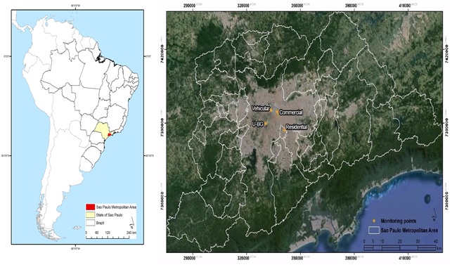Figure 1
Location of the SPMA (left)

Location of the SPMA (left); satellite image and political boundaries of the SPMA with the location of CETESB air quality monitoring stations used (left)

Source: Satellite image and political boundaries of the SPMA with the location of CETESB.

In this study, we used data from 1996-2011, for all pollutants, except for the commercial site, which has only PM10 and O₃ data starting from 1997. We chose not to further extend our time series because we are relating air pollution to the land use characteristics in the immediate vicinity of the monitoring stations. Because intraurban land use changes in these scales are more likely to be observed over longer periods of time, if we extended the time series, we would also have to assess the land use changes through the same time period around each monitoring point, which would make this study longer and change its scope.

Pollutants weremeasuredhourly using referenced scientific methods – beta radiation for PM₁₀, chemiluminescence for NOx, non-dispersive infrared for CO and ultraviolet radiation for O₃. Data is available freely online by CETESB after a quick subscription in the system at http://qualar.cetesb.sp.gov.br/qualar/home.do . For the larger scale analysis, outgoing longwave radiation (OLR) and surface atmospheric pressure were obtained at Reanalysis 2 (KANAMITSU et al., 2002) for an area representative of the east of the São Paulo state, for which a spatial average was calculated.

The World Health Organization states that decision makers should address different types of urban land use and locations when implementing an air quality network in a given area, in order to gather information about how population is potentially exposed to air pollution inside the city and in its suburbs and also due to the different spatial representativeness of different monitoring sites (WHO, 1999; WHO, 2000; MARTIN et al., 2014). Table 01 shows the four urban land use classes used in this study, which were classified by CETESB following abovementioned criteria, along with the identification of the main traffic roads and vehicle traffic in a 300-m radius around the monitoring points, using the aforementioned documents and data provided by the state Traffic Engineering Company (CET), in a description scheme somewhat similar to the ones used in Briggs et al. (2000) and Vardoulakis et al. (2005). Aerial images showing the different characteristics of each site are shown in Fig. 2.

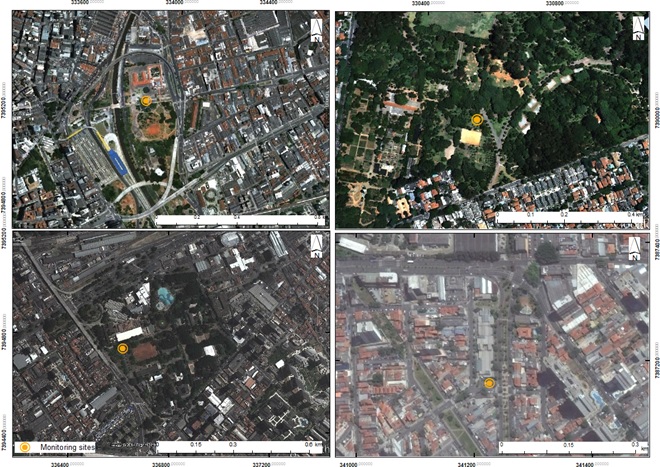Figure 2
Aerial images of the vehicular

Aerial images of the vehicular (top left), U-BG (top right), commercial (bottom left) and residential (bottom right) sites, showing their different characteristics. The monitoring points are indicated by the orange circles

Table 1
Land use classes as suggested by the WHO and characteristics of each site monitored

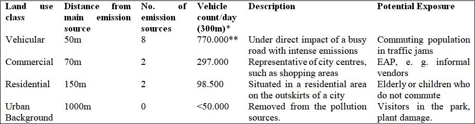
*According to the Traffic Engineering Company.

**Also included total daily trips from the nearby bus terminal.

Diurnal and weekly cycles were calculated by averaging the same hour of the day of the week, in an attempt to capture thehourly variations during the different days of the week for each pollutant in each monitoring point. It was assumed that, in this small scale, the influence of land use would be much stronger than in the other temporal scales. We also performed Pearson’s correlation between the weekly cycles of PM₁₀ and CO, and PM₁₀ and NO₂,which could provide an insight about particulate pollution sources.

For the seasonal analysis, we calculated one single seasonal average for each pollutant at each site by averaging concentrations of three months representative for each season in the Southern Hemisphere: DJF –summer, MAM –autumn, JJA –winter and SON –spring.In order to assess atmospheric seasonality influence over pollutant concentrations, we compared the highest and lowest seasonal average concentrations in the same site and observed this difference in percentage (keepingthe site, varyingthe seasons). In order to assess the urban land useimpact over pollutants, we compared the highest and lowest average concentrations across the different monitoring siteswith different urban land use classes, but in the same season, also in percentage (keepingthe seasons, varyingthe sites). Since atmospheric conditions, in the seasonal scale,are somewhat similar in the metropolitan area, it was assumed that the difference in concentrations were mainly due to atmospheric chemistry changes, induced locally by the exposure/emission/land use characteristics.

Finally, monthly average concentrations of the chosen pollutants were calculated, resulting in monthly time series for the studied period, for comparison with spatially-averaged monthly OLR at 200 mb and surface pressure data for an area encompassing 24.5^◦ to 22.5^◦ S and 45^◦ to 47^◦ W, (east of the Sao Paulo state). Pearson’s correlation coefficients were obtained between OLR and the pollutant monthly averages in each site, in order to analyse if the influence of regional atmospheric systems (which bring cloudiness and atmospheric instability in this region) for the selected pollutants was different at each monitoring point, in a larger temporal scale, according to the land use classes. OLR is an indication of vertical motion and instability in the atmosphere, and as such, could influence pollutant dispersion conditions. A quality control was implemented following the methodology described in Chiquetto and Silva, (2010). For monthly averages, at least 20 days of valid data were necessary, otherwise the month was flagged as invalid, and for the daily averages, if more than 8 hours of the day were invalid, the whole day was flagged as invalid.

3. Results and Discussion

3.1. Weekly and Diurnal cycles

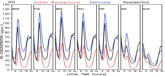
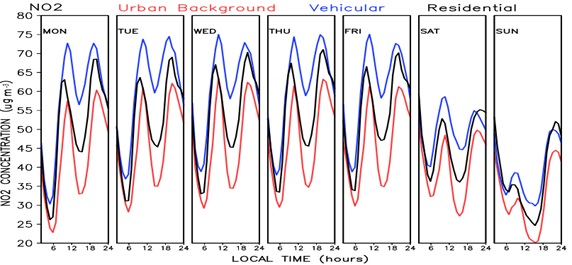
The 16-year diurnal and weekly cycles of the criteria pollutants is shown in figure 3. There are clear differences in the hourly behaviour among the different pollutants analysedaccording to their land use types

Figure 3
Weekly cycle of hourly CO (top), PM₁₀, NO, NO₂ and O₃ (bottom), for the assigned monitoring points (commercial in green, U-BG in red, vehicular in blue, residential in black)

The weekly/diurnal cycle of CO shows higher concentrations and longer peaks in the residential site (around 1.9 ppm), probably due to the predominance of light-duty vehicles activity by the population living in the area, characterized by high income levels, and so, the availability of individual transportation. This makes sense because light-duty vehicles emit much more CO than heavy-duty vehicles. Meanwhile, the vehicular site is more affected by heavy-duty vehicles (Table 1). CO peaks occur twice a day, following the morning and evening rush hour times, as has been observed by other studies (WENG; YANG, 2006) and also in thisstudy area (ROZANTE et al., 2017; CHIQUETTO et al., 2017). In the U-BG site, concentrations are lower (peaking at 1.3 ppm) and there’s a lag of one hour – probably because of advection time, due to the longer distance of the pollution sources. During the afternoon, concentrations decrease due to greater turbulence in the boundary layer from solar heating combined with a decrease in emissions compared to the rush hours. Likewise, concentrations increase after midnight and during early morning hours, probably associated to a lower boundary layer during these hours, after the evening rush hour. On weekends, concentrations decrease substantially (particularly on Sundays), but remain higher in the residential site (indicating substantial urban activity). Also, the peaks occur at night, during hours when people often return or leave home during weekends.

For the particulate pollution, patterns are very different temporally and in each monitoring site, but generally presenting three peaks during the weekdays. Two of these peaks are associated to the morning and evening rush hours are also present, when concentrations are higher in the vehicular site (around 60 µgm^-3), but there are many other sources and factors other than vehicle activity which influence particulate pollution (GIUGLIANO et al., 2005; KULSHRESTHA et al., 2009). In the U-BG site, located inside an urban park, the evening peak is much higher (around 50-55 µgm^-3) than the morning peak, while in the residential and commercial sites, peak concentrations in the morning and evening are generally similar (around 40-50 µgm^-3). For all sites, the midnight/early morning peak is higher than other peaks (60 µgm^-3), probably due to the low boundary layer, except for the U-BG site, where the evening peak is still higher. Also, concerning this site, higher PM₁₀ concentrations are observed during weekends, much higher than in other sites, patterns which are probably associated to the public leisure activities in the park (with more than 200.000 visitors every weekend), which has many bare soil surface areas close to the monitoring point. It may also be the cause of the higher concentrations in the evenings – when people leave work or school and play sports or simply walk and enjoy the park at night. The commercial site, located in an area with mixed land use characteristics inside a school (with bare soil surfaces for sports practices – Fig. 2), also presents higher PM₁₀ concentrations during weekends compared to the vehicular and residential sites. 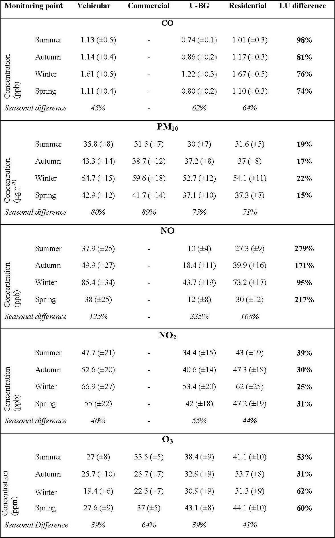Correlation coefficients between the average diurnal cycles of PM₁₀ and CO are of 0.43 for the vehicular site, 0.47 for the residential site and 0.01 for the U-BG site, suggesting that an important part of the particulate pollution could be associated to light vehicle traffic in the first two sites, especially the residential site. Correlations coefficients between PM₁₀ and NO₂, are of 0.26 for the vehicular site, 0.21 for the residential site and 0.18 for the U-BG site, suggesting that the source of particulate pollution can be associated to heavy vehicle traffic in the first two sites, particularly in the vehicular site. Scatterplots are shown in Fig. 04.

Figure 4
Scatterplots of the correlations between the average weekly cycles of CO and PM₁₀ (left) and NO₂ and PM₁₀ (right) for the U-BG, residential and vehicular sites.

For NOx, the weekly/diurnal cycle clearly also shows the peak hours associated to the morning and evening rush hours, with higher values of NO (NO₂) at nearly 130 (75) µgm^-3 at the vehicular site, which is under intense influence of heavy-duty vehicles emissions (Table 1) due to the proximity to many avenues with intense traffic of vehicles, the São Paulo city market and an important bus terminal, which is used by an average of 196.000 people/day, with 61 bus lines, 961 vehicles and 590.000 bus trips/day (CET, 2014 and communication with the City Transport Company). At the U-BG site, NO (NO₂) peaks occur at 50 (60 )µgm^-3, and also later in the day. The residential site shows intermediate concentration levels. It is known that NO₂ has both primary and secondary origins. When emitted by vehicle exhaust, it is actually formed inside vehicle engine via the reaction between NO and oxygen at high temperatures. When formed in the atmosphere, it is via the reaction between NO and O₃ or the oxidation of NO to NO2 via VOCs (BRASSEUR et al., 1999). The morning NO₂ peaks occur later than the NO peaks in all monitoring sites, evidencing the chemical transformation from NO to NO₂. Also, NO₂ concentrations vary less through the day compared to NO and the evening peak is of similar magnitude of the morning peak (unlike NO which shows a much higher morning peak); also, NO₂ concentrations are higher in the U-BG site compared to NO. These results suggest that the secondary parcel of NO2might be more important than the primarily emitted across the megacity (PANDEY et al., 2008; LEVY et al., 2014). During weekends, concentrations of both pollutants decrease significantly in all monitoring sites.

For the ozone averages, there is much less variation throughout the day across the sites. The weekly/diurnal cycle shows peak concentrations (about 90 µgm^-3 in the U-BG site) in the middle of the afternoon on all days, when solar radiation income is maximum and there is availability of precursors emitted in the morning rush hour, as observed in many other locations (BEIG et al., 2007; TANG et al., 2012). There is also an early morning increaseof O₃ at about 4 AM local time in all sites, probably associated to the low boundary layer and greater atmospheric stability in these hours, as observed with other pollutants. Higher concentrations occur in the residential and U-BG sites during the whole week; they are lower in the commercial site and even lower the vehicular site, which is under direct influence of heavy-duty vehicles and has greater NOx concentration, which might end up acting as a sink of O₃. This findings suggests that the removal of O₃ through titration has an important role when defining ozone concentrations locally (GENG et al., 2008), which can be associated to the type and total amount of vehicles in each location (Table 1). The residential site shows highest concentrations at night than other sites. The commercial site, located in an area with mixed land use and intermediate distance to the roads, also shows intermediate O₃ concentration levels. On weekends, concentrations are higher, showing the “weekend effect” which has also been observed in other studies (QIN, 2004; SILVA JÚNIOR et al., 2009; LEVY et al., 2014). The slight increase in ozone at about 4 am is present in all sites and we theorize it could be a likely result from the decrease in the boundary layer height.

Analysis of the hourly standard deviations (data nor shown) indicates that, for all pollutants, temporal variability is higher during the times of maximum diurnal concentration (morning and night for primary pollutants, mid-afternoon for ozone, etc.). This implies that emission conditions also play an important role in the long-term diurnal variability of pollutants. T-student tests were applied to test the difference between pollutant concentrations in the weekly scale in different sites(ex: PM₁₀ at the residential site vs. PM₁₀ at the commercial site, and so on) was found significant for the 99% interval for all tests, except for the difference betweenthe residential and vehicular sites for CO, (95%).

3.2.Seasonal Analysis

In the SPMA, most of the primary pollutants tend to have a distinct seasonal cycle with a minimum during summer (due to greater air instability and precipitation) and a maximum in the more stagnant and dry wintertime conditions (MASSAMBANI; ANDRADE, 1994; CETESB, 2016). For ozone, a minimum occurs from late-autumn to mid-winter, and a maximum in mid-spring, according to the solar radiation seasonal variations in the SPMA (MASSAMBANI; ANDRADE, 1994; CHIQUETTO; SILVA, 2010). Also, local increase of NO during winter could contribute to a greater ozone loss by titration.

Table 2 shows the comparison between the known effects of seasonality and investigated effects of land use in different pollutants. For NO and O₃, the seasonal variation intensity can be compared to that induced by emission/land use characteristics. For NO₂ and PM₁₀, the seasonal variation is much stronger, particularly for the latter, while for CO, land use variations are stronger.

In the commercial site, CO measurements started in 2005, so data is not shown for comparison with other sites (according to other published works, there is a strong decrease in CO concentration in the study area since the last decade (RIBEIRO et al., 2016; ROZANTE et al., 2017), which could cause a bias in the study). CO concentration averages are higher in the residential site, even compared to the vehicular site. Albeit being a less reactive primary pollutant, some studies also show that CO can be impacted by local emission characteristics, showing marked differences in concentration in small spatial scales, of a few blocks (WENG; YANG, 2006). This could be associated to the fact that, in a residential area, the prevailing traffic is from light-duty vehicles (especially in high-income areas, where more people can afford purchasing cars, such as where this station is located), compared to the more heavy-duty-traffic characteristics of the vehicular site studied. This suggests that land use/emission characteristics play an important role in the seasonal scale, and the spatial variations of CO could be stronger than seasonal variations across the megacity. Statistically significant differences for CO were found in all sites investigated, except between the residential and vehicular sites.

Concerning PM₁₀, seasonal differences in each site are much more intense than the land use/emission differences. This could be attributed to the diversity of particulate emission sources, both anthropogenic and natural, such as biomass burning, soil resuspension, marine salt, besides the secondary fraction of the PM formed in different environmental conditions (DE MIRANDA et al., 2012). This suggests that, in the interannual scale, seasonal differences can be much more relevant than spatial variations for this pollutant in this study area (GIUGLIANO et al., 2005; KULSHRESTHA et al., 2009), surely differently from what was observed in the diurnal/weekly scale (Fig. 1). In spite of these findings, statistically significant differences were found between all sites, except between the U-BG and residential sites.

Table 2
Comparison between the influences of land use (bold, far right in each box) and seasonal variations (italic, bottom in each box) in seasonal averages.

However, concerning NO, strong differences concerning both seasonal variation and land use/emission were observed, possibly due to the fact that it is a highly reactive gas. Pandey et al., (2008) observed concentrations 4 times higher in a rural background site compared to a vehicular site. In this study, the difference between the vehicular and the U-BG site is of 277% during summer (nearly thrice as high). As a primary pollutant, its concentrations are lower in the U-BG site, and higher in the other sites, particularly in the vehicular site. Statistically significant differences for NO were found in all sites investigated.

For NO₂, which is less reactive than NO, seasonal differences are more intense than land use/emission differences(albeit less than for PM₁₀).These results reinforce the idea that secondary NO₂ is more relevant across the SPMA than direct NO₂ vehicular emissions. Other regional processes, such as emission from agricultural areas, etc., could also influence seasonal variations of NO₂, particularly at the U-BG site (where seasonal differences are about 55%); this could be further investigated with the use of atmospheric models (PANDEY et al., 2008). Statistically significant differences for NO₂ were found in all sites investigated.

For ozone, in the vehicular, residential and U-BG sites, seasonal differences are approximately 40%. In the commercial site, which presents transitional land use/emission/exposure characteristics, the seasonal variation increases to 64%, showing greater temporal variation compared to other sites. On the other hand, land use/emission variations around each site also influence O₃, with concentrations in the residential site 62% higher than the vehicular during the minimum in winter and 60% higher during the maximum in spring. As discussed previously by the literature (GENG et al., 2008; PANDEY et al., 2008; BIGI; HARRISON, 2010), higher O₃ concentration averages are not observed in sites directly close to the emission sources, with higher urban activity, but in areas with lesser activity (residential) or further away from emissions (U-BG), especially when considering complex megacities. Statistically significant differences in ozone concentrations were found between all sites, except between U-BG and residential.Seasonal averages were also statistically tested in the same way as diurnal/weekly cycles and are significant for the 99% interval, except between the residential and U-BG sites for ozone, which are significant for the 95% interval.

3.3. Monthly means and correlation with regional atmospheric data

Table 3 show the results between the correlations between OLR and the criteria pollutants. Figure 5 shows the strongest correlations (O₃ and MP₁₀). Results are stronger for the U-BG site than the vehicular site, which demonstrates that urban land use plays an important role even when definig the influence of regional atmosphereic systems over pollutant concentrations.

Positive correlationsbetweenregional monthly OLR with PM₁₀ (0.22 to 0.37) in all monitoring sites (table 3) are probably due to the fact that cloudiness is commonly associated to atmospheric instability or low surface pressure in tropics (e.g. precipitation), conditions which tend to increase pollutant dispersion, and also due to its great diversity of sources and also for the environmental-dependent complexity involving secondary aerosol chemistry (LEVY et al., 2014). These correlations are much lower for the primary pollutants (around 0.1) and at the vehicular site (0.22), which are much more directly impacted by emissions, which also suggestthat emission and land use play important roles in pollutant concentrations when considering larger temporal and spatial scales. However, for ozone, stronger correlations with OLR (from 0.33 to 0.48) are probably associated to the fact that cloudiness conditions decrease solar radiation at the surface, and so, hinder photolysis that triggers ozone production (MASSAMBANI; ANDRADE, 1994; CHIQUETTO; SILVA, 2010).

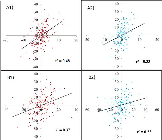Figure 5
Scatterplots showing monthly OLR and ozone correlations

Scatterplots showing monthly OLR and ozone correlations (A1: U-BG, A2: vehicular) and OLR and PM₁₀ (B1 – U-BG and B2 – vehicular).

Table 3
Correlation coefficient between monthly means of OLR at 200 mb, from 1996-2011, and the selected pollutants in the different urban land use classes

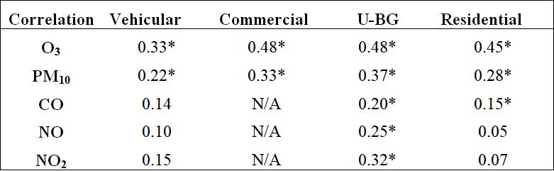
*Statistically significant correlation

Correlations are stronger for all pollutants at the urban U-BG site,which shows more clearly that regional-scale atmospheric conditions exert a stronger influence at the U-BG site compared to other monitoring sites,especially comparing to the vehicular site (Figure 5) (GENG et al., 2008; TANG et al., 2012; LEVY et al., 2014). The residential site shows stronger correlations for ozone, similar to the U-BG site, but also lower for the primary pollutants, similar to the vehicular site, since it is impacted locally by CO emission (Fig. 2, Table 2). Moreover, for O₃ and PM₁₀, correlations were statistically significant in all sites, showing that conditions associated to atmospheric instability on a regional scale impact more on secondary pollutants than on primary pollutants. At the U-BG site, correlations were statistically significant with OLR for all pollutants, including primary pollutants, demonstrating the importance of land use in the temporal variability of pollutants in the intraurban scale.

4. Conclusions and Final Considerations

The objective of this study was to demonstrate the influence of land use in air pollutant concentrations in different land use types within the Sao Paulo megacity, in a range of different time scales from hourly to long-term monthly, in the perspective of complex coupled human-natural systems.Results show that the characteristics of the location of the monitoring site, including distance from pollutant sources (and sinks), density of roads, number of vehicles, surface cover and overall predominant activities (represented by the urban land use class), strongly impact pollutant concentrations and their spatial and temporal variability in all scales of analysis. Urban land use influence is stronger in the diurnal/weekly cycles, particularly for primary pollutants derived from fuel combustion (CO and NO), with concentrations about two to three times higher in the residential sitefor CO (accounting for individual auto use), or in the vehicular site, for NO (heavy vehicle use), compared to the U-BG site. For NO₂ and O₃, the daily amplitudes are less marked than the primary pollutants, showing that concentrations are also influenced by environmental conditions associated to transport and chemical reactions. This also suggests that the secondary fraction of NO₂ is relevant in all urban land use classes and might be so across the megacity of São Paulo. For PM₁₀, the patterns are very diverseon the different days in each monitoring site, associated to its diversity of sources, both human and anthropogenic.Land use strongly influences CO variations in the seasonal scale. However, for O₃ and NO, seasonal differences are as strong as land use/emission differences, and for NO₂ and PM₁₀, seasonal differences are stronger in this scale of analysis, especially for particulate pollution, suggesting the relevance of interannual atmospheric or regional transport processes.In the longer time series and regional analysis, all these differences are less marked, as expected. Nevertheless, they are still presentand statistically significant.

These results demonstrate that, due to the complex mosaic of urban land uses within megacities, the spatial variability of air pollutants are considerably affected by 1) the predominant urban activities, 2) the pollutant considered and 3) the temporal scale of analysis.As one moves towards larger temporal and spatial scales of analysis, air pollution shiftsfrom an anthropogenic to a naturally-inducedsystem, yet the influence of land use is perceived somehow across all scales. This could help policy makers to better plan air quality abatement public policies, when, for example, aiming to attain air quality standards for each pollutant which also have regulations in different time scales (yearly, daily, etc.). It also suggests that the spatial variability ofpollutant concentrations can be complex in such environments, particularly for shorter time scales. Finally, these findings may have implications for future decision-making and environmental, public health and transportation policies for similar megacities involving land use change when considering air quality problems. For example, it is expected that ozone concentrations will increase in areas where city parks or other pedestrian-friendly structures are to be built if they are bordered by important roads with significant precursors emission, exposing the commuting or visiting population to higher ozone concentrationswithin megacities, especially should the fuel use shifts from gasoline to ethanol, demonstrating the complexity of interchanges between human and natural components within a megacity system.

5. References

ALVIM D.S.; GATTI L.V.; CORRÊA S.M.; CHIQUETTO J.B.; DE SOUZA ROSSATTI C.; PRETTO A.; DOS SANTOS M.H.; YAMAZAKI A.; ORLANDO J.P.; SANTOS G.M. Main ozone-forming VOCs in the city of Sao Paulo: observations, modelling and impacts. Air Quality, Atmosphere & Health. New York, v. 10, n.4, p. 421-435, 2016. https://doi.org/10.1007/s11869-016-0429-9

AMANN M.; DERWENT, D.; FORSBERG, B.; HÄNNINEN, O.; HURLEY, F.; KRZYZANOWSKI, M.; DE LEEUW, F.; LIU, S. J.; MANDIN, C.; SCHNEIDER, J.; SCHWARZE, P.; SIMPSON, D. Health risks of ozone from long-range transboundary air pollution. Copenhagen: World Health Organization Regional Office for Europe, 2008.

AMORIM, M. C. C. T. Climatologia e Gestão Do Espaço Urbano. Mercator. Fortaleza, v. 9, n.1, p.71-90, 2011. https://doi.org/10.4215/RM2010.0901.0005

ANDERSON, L. G. Ethanol fuel use in Brazil: air quality impacts. Energy & Environmental Science. London. v. 2, n. 10, p. 1015, 2009. https://doi.org/10.1039/b906057j

BAKLANOV, A.; MOLINA, L. T.; GAUSS, M. Megacities, air quality and climate. Atmospheric Environment. Amsterdam, n. 126, p. 235–249, 2016. https://doi.org/10.1016/j.atmosenv.2015.11.059

BARROS, J. R.; ZAVATTINI, J. A. Bases conceituais em climatologia geográfica (theconceptual bases in geographicalclimatology). Mercator. Fortaleza, v. 8, n. 16, p. 255-26, 2009. https://10.4215/RM2009.0816.0019

BEIG, G., GUNTHE, S., JADHAV, D. B. Simultaneous measurements of ozone and its precursors on a diurnal scale at a semi urban site in India. Journal of Atmospheric Chemistry. Amsterdam, v. 57, n. 3, p. 239–253, 2007. https://doi.org/10.1007/s10874-007-9068-8

BIGI, A.; HARRISON, R. M. Analysis of the air pollution climate at a central urban background site. Atmospheric Environment. Amsterdam, v. 44, n. 16, p. 2004–2012, 2010. https://doi.org/10.1016/j.atmosenv.2010.02.028

BRASSEUR, G., et al. Atmospheric chemistry and global change. Oxford, Oxford University Press, 1999.

BRAVO, M. A.; SON, J.; DE FREITAS, C. U.; GOUVEIA, N.; BELL, M. L. Air pollution and mortality in Sao Paulo, Brazil: Effects of multiple pollutants and analysis of susceptible populations. Journal of Exposure Science and Environmental Epidemiology. Berlin, v. 26, n. 2, p. 150–161, 2016. https://doi.org/10.1038/jes.2014.90

BRIGGS, D. J.; DE HOOGH, C.; GULLIVER, J.; WILLS, J.; ELLIOTT, P.; KINGHAM, S.; SMALLBONE, K. A regression-based method for mapping traffic-related air pollution: application and testing in four contrasting urban environments. Science of the Total Environment. Amsterdam, v. 253, n. 1–3, p. 151–167, 2000. https://doi.org/10.1016/S0048-9697(00)00429-0

CET – Companhia de Engenharia de Tráfego. Pesquisa de Fluidez –Desempenho do Sistema Viário Principal: Volume e Velocidade – 2013. São Paulo, Diretoria Adjunta de Planejamento, Projetos e Educação de Trânsito – DP, 2014.

CETESB – Companhia Ambiental do Estado de São Paulo. Relatório Anual da Qualidade do Ar do Estado de São Paulo, 2015. São Paulo: Divisão de Análise de dados, 2016.

CHAMEIDES, W. L.; FEHSENFELD, F.; RODGERS, M. O.; CARDELINO, C.; MARTINEZ, J.; PARRISH, D.; WANG, T. Ozone precursor relationships in the ambient atmosphere.Journal of Geophysical Research. Washington DC, v. 97(D5), p. 6037-6055, 1992. https://doi.org/10.1029/91JD03014

CHIQUETTO, J. B.; SILVA, M. E. S. Sao Paulo’s “Surface Ozone Layer” and the Atmosphere. Saarbrücken, VDM Verlag Dr Müller, 2010.

CHIQUETTO, J. B.; SILVA, M. E. S.; CABRAL-MIRANDA, W.; RIBEIRO, F. N. D.; IBARRA-ESPINOSA, S. A. ; YNOUE, R. Y. Air Quality Standards and Extreme Ozone Events in the São Paulo Megacity. Sustainability, v. 11, p. 3725, 2019. https://doi.org/10.1016/j.atmosenv.2017.03.051

CHIQUETTO, J. B.; YNOUE, R.; CABRAL-MIRANDA, W.; SILVA, M. E. Concentrações de ozônio troposférico na Região Metropolitana de São Paulo e a implementação de parques urbanos: observações e modelagem [Concentrations of Tropospheric Ozone in the Metropolitan Area of São Paulo and theimplementation of Urban Parks]. Boletim Paulista de Geografia. São Paulo, n. 95,p 1-24, Jan. 2017, SpecialIssue. Available online: https://agb.org.br/publicacoes/index.php/boletim-paulista/article/view/668. Accessed on: 20/03/2020.

CHRISTOFOLETTI, A.Modelagem de Sistemas Ambientais. Edgard Blücher, 1999.

DE MIRANDA, R. M.; DE FATIMA ANDRADE, M.; FORNARO, A.; ASTOLFO, R.; DE ANDRE, P. A.; SALDIVA, P. Urbanairpollution: a representativesurveyof PM2.5 massconcentrations in sixBraziliancities. Air Quality, Atmosphere & Health. New York, v. 5, n. 1, p. 63–77, 2012. https://doi.org/10.1007/s11869-010-0124-1

FREITAS, E. D.; ROZOFF, C. M.; COTTON, W. R.; DIAS, P. L. S. Interactions of an urban heat island and sea-breeze circulations during winter over the metropolitan area of São Paulo, Brazil. Boundary-Layer Meteorology, New York, v. 122, n. 1, p. 43–65, 2007. https://doi.org/10.1007/s10546-006-9091-3

GENG, F.; TIE, X.; XU, J.; ZHOU, G.; PENG, L.; GAO, W.; ZHAO, C. Characterizations of ozone, NOx, and VOCs measured in Shanghai, China. Atmospheric Environment. Amsterdamv. 42, n. 29, p. 6873–6883, 2008. http://doi.org/10.1016/j.atmosenv.2008.05.045

GIUGLIANO, M.; LONATI, G.; BUTELLI, P.; ROMELE, L.; TARDIVO, R.; GROSSO, M. Fine particulate (PM2.5PM1) at urban sites with different traffic exposure. Atmospheric Environment. Amsterdam,v. 39, n. 13, p. 2421–2431, 2005. https://doi.org/10.1016/j.atmosenv.2004.06.050

GONÇALVES, F. L. T.; CARVALHO, L. M. V.; CONDE, F. C.; LATORRE, M. R. D. O.; SALDIVA, P. H. N.; BRAGA, A. L.The effects of air pollution and meteorological parameters on respiratory morbidity during the summer in São Paulo City. Environment International. Amsterdam, v. 31, n. 3, p. 343–349, 2005. https://doi.org/10.1016/j.envint.2004.08.004

GURJAR, B. R.; JAIN, A.; SHARMA, A.; AGARWAL, A.; GUPTA, P.; NAGPURE, A. S.; LELIEVELD, J. Human health risks in megacities due to air pollution. Atmospheric Environment. Amsterdam, v. 44, n. 36, p. 4606–4613, 2010. https://doi.org/10.1016/j.atmosenv.2010.08.011

JOHNSON, M.; ISAKOV, V.; TOUMA, J. S.; MUKERJEE, S.; OZKAYNAK, H. Evaluation of land-use regression models used to predict air quality concentrations in an urban area. Atmospheric Environment, Amsterdam, v. 44, n. 30, p. 3660–3668, 2010. https://doi.org/10.1016/j.atmosenv.2010.06.041

KANAMITSU, M., EBISUZAKI, W., WOOLLEN, J., YANG, S.-K., HNILO, J. J., FIORINO, M., POTTER, G. L. NCEPDOE AMIP-II Reanalysis (R-2). Bulletin of the American Meteorological Society. Boston, v. 83, n. 11, p. 1631–1643, 2002. https://doi.org/10.1175/BAMS-83-11-1631

KRAAS F.; MERTINS G. Megacities and global change. In: KRAAS, F.; AGGARWAL, S.; COY, M.; MERTINGS, G. Megacities: Our Global Urban Future. Dordrecht: Springer, 2014, p 1-6.

KULSHRESTHA, A.; SATSANGI, P. G.; MASIH, J.; TANEJA, A. Metal concentration of PM2.5 and PM10 particles and seasonal variations in urban and rural environment of Agra, India. Science of The Total Environment. Amsterdam, v. 407, n. 24, p. 6196–6204, 2009. https://doi.org/10.1016/j.scitotenv.2009.08.050

LEVY, I.; MIHELE, C.; LU, G.; NARAYAN, J.; HILKER, N.; BROOK, J. R. Elucidating multipollutant exposure across a complex metropolitan area by systematic deployment of a mobile laboratory. Atmospheric Chemistry and Physics. Göttingen, v. 14, n. 14, p. 7173–7193, 2014. https://doi.org/10.5194/acp-14-7173-2014

LIU, J., DIETZ, T., CARPENTER, S. R., ALBERTI, M., FOLKE, C., MORAN, E., … TAYLOR, W. W. Complexity of Coupled Human and Natural Systems. Science. Washington DC, n. 317, v. 5844, p. 1513–1516, 2007. https://doi.org/10.1126/science.1144004

MARTIN, F.; FILENI, L.; PALOMINO, I.; VIVANCO, M. G.; GARRIDO, J. L. Analysis of the spatial representativeness of rural background monitoring stations in Spain. Atmospheric Pollution Research. Amsterdam, v. 5, n. 4, p. 779–788, 2014. https://doi.org/10.5094/APR.2014.087

MARTINS, M. H. R. B.; ANAZIA, R.; GUARDANI, M. L. G.; LACAVA, C. I. V.; ROMANO, J.; SILVA, S. R. Evolution of air quality in the Sao Paulo metropolitan area and its relation with public policies. International Journal of Environment and Pollution. Geneva, v. 22, n. 4, p. 430, 2004. https://doi.org/10.1504/IJEP.2004.005679

MASSAMBANI, O.; ANDRADE, M. F. Seasonal behavior of tropospheric ozone in the Sao Paulo (Brazil) metropolitan area. Atmospheric Environment. Amsterdam, v. 28, n. 19, p. 3165–3169, 1994. https://doi.org/10.1016/1352-2310(94)00152-B

MENDONÇA, F. SAU – Sistema Ambiental Urbano: uma abordagem dos problemas socioambientais da cidade. Curitiba. Editora da UFPR, 2004.

MOLINA, M. J.; MOLINA, L. T. Megacities and Atmospheric Pollution. Journal of the Air & Waste Management Association. Abingdon-on-Thames, v. 54, n. 6, p. 644–680, 2004. https://doi.org/10.1080/10473289.2004.10470936

PANDEY, S. K.; KIM, K.-H.; CHUNG, S.-Y.; CHO, S.-J.; KIM, M.-Y.; SHON, Z.-H. Long-term study of NOx behavior at urban roadside and background locations in Seoul, Korea. Atmospheric Environment. Amstedam,v. 42, n. 4, p. 607–622, 2008. https://doi.org/10.1016/j.atmosenv.2007.10.015

Plano Diretor Estratégico – São Paulo. Aprova a Política de Desenvolvimento Urbano e o Plano Diretor Estratégico do Município de São Paulo e revoga a Lei no 13.430/2002. São Paulo, 2014. Available online: http://www.prefeitura.sp.gov.br/cidade/secretarias/upload/chamadas/2014-07-31_-_lei_16050_-_plano_diretor_estratgico_1428507821.pdf. Accessed on 17/06/2019.

PUJADES-RODRIGUEZ, M.; MCKEEVER, T.; LEWIS, S.; WHYATT, D.; BRITTON, J.; VENN, A. Effect of traffic pollution on respiratory and allergic disease in adults: cross-sectional and longitudinal analyses. BMC Pulmonary Medicine. Berlin, v. 9, n. 1, p. 42, 2009. https://doi.org/10.1186/1471-2466-9-42

QIN, Y. Weekend/weekday differences of ozone, NOx, Co, VOCs, PM10 and the light scatter during ozone season in southern California. Atmospheric Environment. Amsterdam, v. 38, n; 19, p. 3069–3087, 2004. https://doi.org/10.1016/j.atmosenv.2004.01.035

RIBEIRO, F. N. D.; SALINAS, D. T. P.; SOARES, J.; DE OLIVEIRA, A. P.; DE MIRANDA, R. M.; SOUZA, L. A. T. The Evolution of Temporal and Spatial Patterns of Carbon Monoxide Concentrations in the Metropolitan Area of Sao Paulo, Brazil. Advances in Meteorology. London,v. 2016, p. 1–13, 2016. https://doi.org/10.1155/2016/8570581

ROZANTE, J.; ROZANTE, V.; SOUZA ALVIM, D.; OCIMAR MANZI, A.; BARBOZA CHIQUETTO, J.; SIQUEIRA D'AMELIO, M.; MOREIRA, D. Variations of Carbon Monoxide Concentrations in the Megacity of Sao Paulo from 2000 to 2015 in Different Time Scales. Atmosphere. Basel, v. 8, n. 5, p. 81, 2017. https://doi.org/10.3390/atmos8050081

SEINFELD, J. H.; PANDIS, S. N. Atmospheric chemistry and physics: from air pollution to climate change. 3rd edition. Hoboken, 2016.

SILVA, G.; FONSECA, M. L. São Paulo, city-region: constitution and development dynamics of the São Paulo macrometropolis. International Journal of Urban Sustainable Development. Abingdon-on-Thames, v. 5, n.1, p. 65–76, 2013. https://doi.org/10.1080/19463138.2013.782707

SILVA JÚNIOR, R. S. DA; OLIVEIRA, M. G. L.; ANDRADE, M. F. Weekend/weekday differences in concentrations of ozone, nox, and non-methane hydrocarbon in the metropolitan area of São Paulo. Revista Brasileira de Meteorologia. São José dos Campos, v. 24, n.1, p. 100–110, 2009. https://doi.org/10.1590/S0102-77862009000100010

SZPIRO, A. A.; SAMPSON P. D.; SHEPPARD, L.; LUMLEY, T.; ADAR, S. D.; KAUFMAN, J. D. Predicting intra‐urban variation in air pollution concentrations with complex spatio‐temporal dependencies. Environmetrics. Hoboken, v. 21, n. 6, p. 606-631, 2010. https://doi.org/10.1002/env.1014

TANG, G.; WANG, Y.; LI, X.; JI, D.; HSU, S.; GAO, X. Spatial-temporal variations in surface ozone in Northern China as observed during 2009–2010 and possible implications for future air quality control strategies. Atmospheric Chemistry and Physics, 12(5), 2757–2776, 2012. https://doi.org/10.5194/acp-12-2757-2012

TSAO, C. C.; CAMPBELL, J. E.; MENA-CARRASCO, M.; SPAK, S. N.; CARMICHAEL, G. R.; CHEN, Y. Increased estimates of air-pollution emissions from Brazilian sugar-cane ethanol. Nature Climate Change, 2(1), 53–57, 2011. https://doi.org/10.1038/nclimate1325

UN. World urbanization prospects, the 2014 revision: highlights. New York, 2014. Available online: http://proxy.uqtr.ca/login.cgi?action=login&u=uqtr&db=ebsco&ezurl=http://search.ebscohost.com/login.aspx?direct=true&scope=site&db=nlebk&AN=857993. Accessed on: 30/03/2020.

VARDOULAKIS, S.; GONZALEZFLESCA, N.; FISHER, B.; PERICLEOUS, K. Spatial variability of air pollution in the vicinity of a permanent monitoring station in central Paris. Atmospheric Environment, 39(15), p. 2725–2736, 2005. https://doi.org/10.1016/j.atmosenv.2004.05.067

WANG, Y.; KONOPKA, P.; LIU, Y.; CHEN, H.; MULLER, R.; PLOGER, F., … LU, D. Tropospheric ozone trend over Beijing from 2002-2010: ozonesonde measurements and modeling analysis. Atmospheric Chemistry and Physics. Göttingen, v. 12, n. 18, p. 8389–8399, 2012. https://doi.org/10.5194/acp-12-8389-2012

WENG, Q.; YANG, S. Urban Air Pollution Patterns, Land Use, and Thermal Landscape: An Examination of the Linkage Using GIS.Environmental Monitoring and Assessment. Amsterdam, v. 117, n. 1–3, p. 463–489, 2006. https://doi.org/10.1007/s10661-006-0888-9

WHO (Ed.). Monitoring ambient air quality for health impact assessment. Copenhagen: World Health Organization, Regional Office for Europe, 1999. Available online: https://apps.who.int/iris/bitstream/handle/10665/107332/E67902.pdf?sequence=1&isAllowed=y. Accessed on 09/03/2020.

WHO (Ed.). Air quality guidelines for Europe. 2. ed. Copenhagen: World Health Organization, Regional Office for Europe, 2000. Available online: https://apps.who.int/iris/bitstream/handle/10665/107335/E71922.pdf?sequence=1&isAllowed=y. Accessed on 12/12/2019.

YUVAL; BRODAY, D. M. High-resolution spatial patterns of long-term mean concentrations of air pollutants in Haifa Bay area. Atmospheric Environment. Amsterdam,v. 40, n. 20, p. 3653–3664, 2006. https://doi.org/10.1016/j.atmosenv.2006.03.037

Author notes