

Artículos
DEPENDENCE OF LATIN AMERICA EXTERNAL SECTOR ON COMMODITY PRICES. A CONTEMPORANEITY ANALYSIS USING STRUCTURAL BREAKS
Revista Económica La Plata
Universidad Nacional de La Plata, Argentina
ISSN: 1852-1649
Periodicity: Anual
vol. 65, 2019
Received: 01 October 2018
Accepted: 20 December 2019
Corresponding author: Fernando.delbianco@uns.edu.ar

Abstract:
We seek to analyze the relationship between some macroeconomic variables and commodity prices in Latin America. The main hypothesis is that the economic performance in the area is tied to the pattern followed by the commodity prices. Moreover we expect to find that some commodities are more relevant than others. We find evidence supporting our former hypothesis but not the latter. An important result is that macroeconomic variables and commodity prices breaks followed a bimodal distribution over the last 60 years with one mode around the 70s and the other mode at the beginning of the 21th century.
JEL classification: C12;
C58; E44; F44.
Keywords: Commodities dependence, external sector, Latin America, breaks estimation.
Resumen:
En el presente trabajo analizamos la relación entre determinadas variables macroeconómicas y los precios de commodities en América Latina. La hipótesis principal es que el desempeño económico del área siguió el patrón del movimiento de los precios de las commodities. También era esperable que algunas commodities fuesen más relevantes que otras. Encontramos evidencia a favor de nuestra primera hipótesis, pero no de la segunda. Un resultado importante es que los quiebres de las variables económicas y de los precios de las commodities siguieron una distribución bimodal durante los últimos 60 años con una moda en los setentas y la otra moda a principios del siglo 21.
Clasificación
JEL : C12; C58; E44; F44.
Palabras clave: Dependencia de commodities, sector externo, América Latina, estimación de quiebres.
I. Introduction
In this paper we pose a simple question from a descriptive point of view: Did changes on the trends of the external sector of Latin American countries take place at the same time as changes on worldwide commodity price indexes? More explicitly, we obtain breaks on different series of the external sector and commodity price indexes of the countries of Latin America and compare the dates looking for contemporaneity. If they were indeed contemporaneous we can argue that there is some sense of dependence of the external sector on commodities since the former is sensitive to the latter.
We based our study on the papers published in “Los recursos naturales como palanca del desarrollo en América del Sur: ¿ficción o realidad?” (“Natural resources as trigger of growth in South America: fiction or reality?”) Edited by Red Mercosur, especially the work done by Albrieu.
The author uses as a part of his analysis of data on commodities estimations based on exogenous breaks that he considers relevant to include and test. In our paper we use a series of endogenous break tests to figure out when commodity price indexes had suffered a break and we compare those with the breaks on the macroeconomic variables of each country in Latin America, more specifically we compare those breaks with the current account and external sector variables such as exports and imports. Since our focus is on the external sector we do not use any measure of GDP or GDP growth.
Regarding some stylized facts it can be mentioned that during the 21st century a new growth path was introduced in the world which was different to the ones followed worldwide before. Particularly some strong new players came into play such as China (Gallagher and Porzecanski, 2010), India and other players that were already important but became more prominent like Brazil and Russia. In other words, the emerging world became a fundamental actor in the new setup not only because of the crises suffered by the developed countries (mainly after Lehman Brothers) but also after the new trade links between developing countries were settled (south-south trade). In this new world, after the BRICs (Brazil, Russia, India and China) a new group is gaining power: the MINTs (Mexico, Indonesia, Nigeria and Turkey).
In particular, when we look at Latin America we can observe very high economic growth in the last decade in comparison to what had happened throughout the second half of the 20th century (the former experience is known in everyday language as “growing at Chinese rates”).
The key of the success of these economies was the high price of commodities (from soya to oil) that took place after China and India started pushing upwards the demand of these goods.
As Albrieu (2012) mentions:
“The success of a development strategy based on natural resources will not be neutral to the trend and the volatility of the external sector prices: if we follow a declining path on the terms of trade we will have an external deficit and that could undermine the economic growth (Rodríguez, 2006) while high volatility on raw materials prices can increase the macroeconomic instability and through this channel it can reduce economic growth (Lederman and Xu, 2009).”
As it can be seen following a growth path based on the historically high prices of commodities can result in deep problems if the trend stops. Several papers (Fernández et al. (2017); Shousha (2016); Fernández et al. (2018)) point out that around one third of the fluctuations of the economic cycle can be explained by shocks on commodity prices. Albrieu (2012) provides data showing that countries in the region receive between 11% and 33% of their income from selling commodities. Also these countries may be in trouble if public expenditure increases in a higher proportion than the increase of the commodity prices.
At the same time exporting natural resources generates an extra risk: the appreciation of the local currency driven by the increase on the flow of foreign currency toward the country. This effect can trigger several political problems known as “Dutch diseases” (Corden, 1984).
Another study strongly related to our main idea is the paper written by Jaramillo et al. (2009). The authors state that China pushed up the commodity prices and this effect led to an increase on the external sector of Latin American countries. Implicitly they assume that the economic cycles in Latin America are correlated with commodity prices cycles.
We based our work on Hamilton (2008). In his paper he tries to explain the dependence of the US on oil prices because he observes that 9 out of 10 US recessions were preceded by a spike up on oil prices. Although he does not perform any break test he uses the descriptive approach to settle the question. Since he tries to measure the dependence of the US on oil prices using OLS his approach is radically different than ours. While doing this kind of analysis you can explain more formally the shape of the effect it is econometrically difficult to estimate, and noise will tend to increase the likelihood of coefficients statistically not different from zero. To avoid this kind of issues we try to focus on the descriptive stage and to provide a formal benchmark to analyze it.
Several recent papers, including Shousha (2016), Fernández, Schmitt-Grohé and Uribe (2018) and Ben Zeev, Pappa and Vicondoa (2017), conclude that shocks on commodity prices have explanatory power of the cycle of Latin American economies. We differ from these works by using a different methodology to show the relationship between commodity prices and the external sector of Latin American economies that allow us to use a longer dataset.
The authors previously performed a study of cointegration with breaks between commodity prices and current account for Argentina (Delbianco-Fioriti, 2014) and another work extending the results to countries of Latin America and the Caribbean (Delbianco-Fioriti, 2018). In these works evidence suggests that there is a strong relationship between the volatility of commodity prices and the financial flows of the Latin-American region.
We do no state that our channel is the only one that prevails. For example, Ghimire et al. (2016) show that developing countries need aid-for-trade to improve their trade balance, being this channel a relevant one for the countries we consider. Regarding volatility Edwards (2010) finds that regional free trade agreements lower growth volatility. We may contribute to his paper by showing that controlling growth volatility by commodity prices volatility may lead to different conclusions.
The approach in this work is as follows: As a first step we estimate separately breaks on each of the chosen series (current account, trade balance, imports, exports, soya price index, agriculture price index, metals price index, energy price index and not energy price index). Afterwards we plot the results in order to find similarities, which are evident in this exercise. Finally, we look for contemporaneous breaks in order to understand if the external sector is related to commodity prices.
The paper is divided as follows: Section 2 briefly introduces the methodology used. Section 3 presents the results of the paper after detailing the datasets used. Section 4 highlights some conclusions and proposes further research to be done.
II. Methodology
In this section we explain our main structural break test. In the Appendix we show that conclusions are robust to using other tests.
II.1 Bai - Perron (BP)
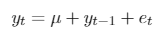
Bai and Perron (1998) consider the following model:
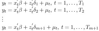 [1]
[1]The dependent variable, observed at the t period, is yt. Covariate vectors are xt(p × 1) and zt(p × 1) and their coefficients vectors are β and δj(j = 1,...,m + 1). µtdenotes the error component, while (T1,T2,...,Tm+1) are the structural breaks, which are treated as unknown.
If p = 0, the model becomes a pure structural break model. Denoting the diagonal matrix = diag(Z1,...,Zm+1), where , the model can be rewritten as follows:
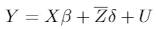 [2]
[2]where , , , and is the diagonal matrix that introduces the breaks at (T1,...,Tm) .
Superscript 0 refers to the real data, so that the data generating process is given by:
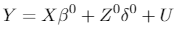 [3]
[3]The goal of the test is to estimate the break points so as to minimize the sum of squared residuals, ST:
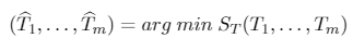 [4]
[4]III. Data and results
Are the comparative advantages of Latin America their curse? Having neither a model nor an idea of causality we try to address how far Latin America depends on commodities, mainly considering the performance of the region at the beginning of the 21st century. Our preliminary hypothesis is that the growth path of these countries is heavily dependent on the trend of the commodities markets. As pointed out by Albrieu (2012), the average share of commodities in the total exports of the countries in the region is 43%. As a first approach we look how close in time are the structural breaks on four of the main macroeconomic variables of the external sector for the Latin American countries with the breaks experienced by the commodity prices.
Our second hypothesis is a decomposition of the first one: if countries do not depend on the commodities as a whole, do they depend on their main produced commodity (such as metals in Chile or agriculture in Argentina)? We pose this question because it is usually considered that these commodities drive the economic cycles on the economies considered and by addressing the issue we could validate the idea or not. As a complement to our contemporary analysis we provide Table A.12 in the appendix highlighting the main commodities for each country obtained from a regression in which it can be seen that in most cases commodities are significant in order to explain the external sector (even though we only provide the relationship between commodities and the current account, we can extend our analysis and obtain similar results).
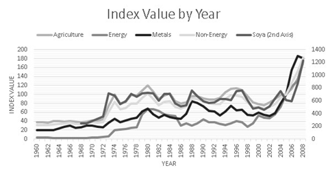
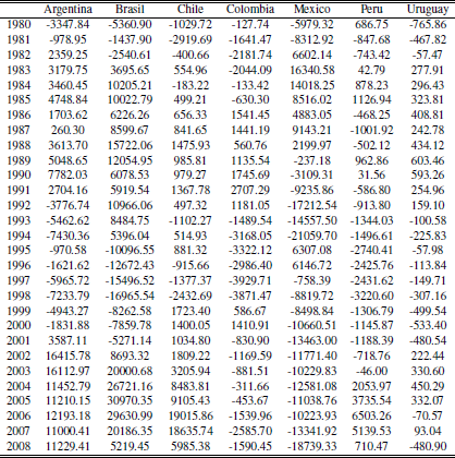
The dataset published by CEPAL (Cuadernillo 37) provides data from 1950 until 2008 about the external sector measured with constant prices. Table A.11 shows the trade balance of the bigger countries for the period 19802008 measured with constant prices of 2000. Also we used several commodity prices indexes (IMF). The indexes correspond to the prices of soya, agriculture in general, energy, not energy and metals. Among those indexes only soya represents a single good while the others represent a bundle of commodities. Since we use a price index, it is expressed in relative terms thus deflating it becomes redundant. We present figure 3 in the appendix showing the commodity indexes path. The macroeconomic variables chosen for the Latin American economies were current account, trade balance, imports and exports. The countries analyzed were Argentina, Bolivia, Brazil, Chile, Colombia, Ecuador, Mexico, Paraguay, Peru, Uruguay and Venezuela.
Our focus is on the external sector of the countries since we want to shed light on the fact that the region used commodities as a mean to obtain foreign currency and foster growth. Another alternative is to examine the relationship between GDP and commodity prices, but many other variables have to be used and the effect is more difficult to observe.
We focused our analysis on understanding how the current account is affected by breaks on the commodities but given the debt episode that took place on these countries on the 80s1 we used as a complement the trade balance because it does not include debt interest’s payment. On the other hand, analyzing exports and imports allows us to see how close the dynamics of the external sector to the dynamics followed by the raw materials are.
In terms of results we show the distribution of breaks (number of breaks found by year with all the tests) in the Figures 1 and 2. It can be observed that all the series analyzed have a bimodal distribution of the breaks with mass around two dates: One towards the end of the 70s and the other along the beginning and middle of the first decade of the 21th century which is consistent with the cycles that took place on the region.
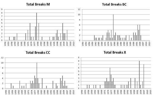
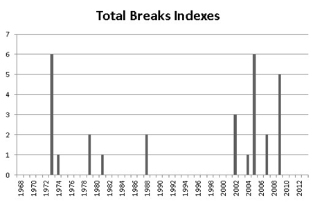
It is interesting to highlight the coincidence of the bimodal distribution between the macro variables and the indexes. There is a slight difference on the mass around each mode that is a consequence of having several macro variables, but the bimodal pattern is obvious. A potential weakness of this result is that some events may have taken place at the same time as the structural breaks (for example liquidity issues or wars) and the results may be misleading, but we can clearly observe some relationship between commodity prices and the external sector of the countries in the area.
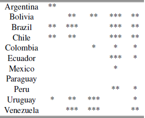
Another way of visualizing the relationship between breaks of commodities and macro variables is counting by year and by country how many macro variables had a break and whether it is contemporary or not with a commodity index break. These results can be observed in the following table.
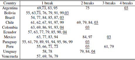
Table 1 highlights the fact that almost every country in the region exhibited a contemporaneity event with a commodity index during the period analyzed (except Venezuela). Similar tables can be obtained for the different break’s methodologies using the tables in the appendix, achieving similar results.
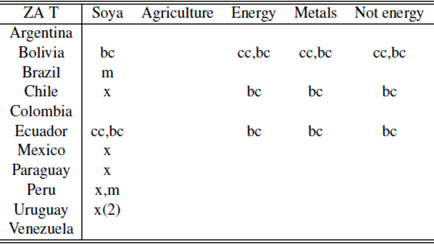
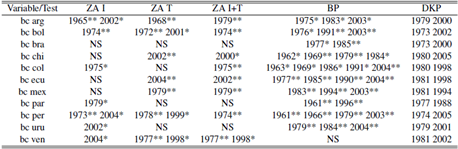
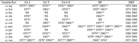
Several figures and tables obtained from the structural break tests are shown in the appendix. After the graphs where the bimodal distribution is present we can see tables detailing by country and by year which macro series were contemporary with which commodity series. The last table lists all the breaks for each variable, by test, and specifies year and significance (KP establishes suggested breaks).
A couple of facts are present in the tables. First, the breaks follow a bimodal distribution as stated before. Moreover there are almost no breaks on the 50s, 60s and 90s. This is even more extreme for the commodities: apart from a suggested break on 1988 there are no breaks outside the 70s and the first decade of the 21th century. This information is available on Tables A.6 to A.10.
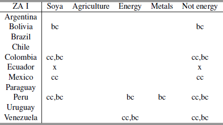
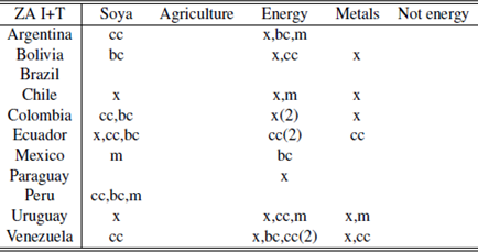
Regarding the contemporaneity Tables (A.1 to A.5), it can be seen a discrepancy of results depending on the test considered (we do not consider contemporaneity between tests). Using ZA with intercept and ZA with trend there are many coincidences between the breaks of soya and energy and some cases among metals and not energy. In most of the countries these breaks coincide with breaks on the trade balance and on the current account and in some cases they are also contemporary with breaks on the exports.
In the case of ZA with intercept and trend not energy becomes irrelevant while energy and agriculture have many cases of contemporaneity. Also, for the case of energy, there are cases where up to three macro variables are contemporaneous with the break.
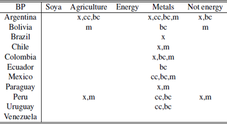
Metals become extremely relevant for the BP test, mainly by being contemporaneous with the trade balance and the current account.
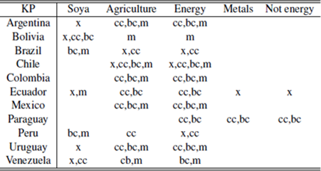
Finally, the KP test (presumably the most powerful given it is more modern) finds many cases of contemporaneity, mainly in agriculture and energy and a few on soya. Moreover, it is important to highlight that this test finds that the commodities breaks are contemporaneous in some cases with the four macro variables chosen in this paper.
As a general final remark it cannot be stated that the main commodities are the ones that drive contemporaneity since metals index is not always contemporaneous for Chile, agriculture is not always for Argentina and Brazil, energy is not always for Bolivia and the same holds true for the remaining countries. This remark shows that our methodology is powerful in terms of contemporaneous events but does not provide enough insight on the degree of dependence.
IV. Conclusions
As a conclusion it can be mentioned that there seems to be a strong relationship between the macroeconomic variables of Latin American countries and the price of the commodities and if this relationship is forgotten then any change on the trend of prices could undermine the growth pattern in the area leaded by the external sector.
The most striking fact on this paper is that macroeconomic variables in Latin America and commodity prices have followed a bimodal distribution. Also, the two modes of both distributions seem to be quite close, highlighting the fact that the area seems to be heavily related to commodity prices.
Some extensions could be to study the correlation to understand if commodity prices break determine macroeconomic variables breaks or the other way around. Another interesting topic is to determine to what extent these economies rely on commodities and to understand the industrialization patterns throughout the period analyzed in this paper.
References
Albrieu, R. (2012), “La Macroeconomía de los recursos naturales en América Latina”, in “Los recursos naturales como palanca del desarrollo: ficción o realidad?”, Red Mercosur.
Bai, J. and P. Perron (1998), “Estimating and Testing Linear Models with Multiple Structural Changes”, Econometrica 66, 47-78.
Bai, J. (1997), “Estimating multiple breaks one at a time”, Econometric Theory 13(3), 315-352.
Bai, J. and P. Perron (2003a), “Critical values for multiple structural change tests,” Econometrics Journal 6, 72-78.
Bai, J. and P. Perron (2003b), “Computation and Analysis of Multiple Structural Change Models”, Journal of Applied Econometrics 18, 1-22.
Bai, J. and P. Perron (2006), “Multiple Structural Change Models: A Simulation Analysis”, in Econometric Theory and Practice: Frontier of Analysis and Applied Research (Essays in Honor of Peter Phillips), ed. by Corbae D., S. Durlauf and B.E. Hansen, Cambridge University Press.
Banerjee, A. and G. Urga (2005), “Modelling structural breaks, long memory and stock market volatility: an overview”, Journal of Econometrics 129, 1-34.
Ben Zeev, N., E. Pappa and A. Vicondoa (2017), “Emerging economies business cycles: The role of commodity terms of trade news”, Journal of International Economics 108, 368-376.
Clemente, J., A. Montanes and M. Reyes (1998), “Testing for a unit root in˜ variables with a double change in the mean”, Economics Letters 59, 175-182.
Corden, W. M. (1984), “Booming Sector and Dutch Disease Economics: Survey and Consolidation”, Oxford Economic Papers, Oxford University Press, 36(3), 359-80, November.
Dickey, D. and W. Fuller (1984), “Testing for unit roots in seasonal time series”, Journal of the American Statistical Associations 79, 355-367.
Delbianco, F. and A. Fioriti (2014) “The impact of commodities indexes in Argentina: A cointegration analysis with breaks”, The empirical economics letters 13(11).
Delbianco, F. and A. Fioriti (2018) “Dependence of Latin America on commodity prices. A contemporaneity analysis”, Lecturas de Economía 88(1), 9-33.
Edwards, J. (2010), “GDP Growth Volatility and Regional Free Trade Agreements”, Applied Econometrics and International Development 10(2), 7386.
Fernández, A., S. Schmitt-Grohé and M. Uribe (2017) “World shocks, world prices, and business cycles: An empirical investigation”, Journal of International Economics 108, S2-S14.
Fernández, A., A. González and D. Rodríguez (2018) “Sharing a ride on the commodities roller coaster: Common factors in business cycles of emerging economies”, Journal of International Economics 111, 99-201.
Frenkel, R. and M. Rapetti (2011), “La principal amenaza de América Latina en la próxima década: ¿fragilidad externa o primarización?”, Mimeo, CEPAL.
Gallagher, K. and R. Porzecanski (2010), “The Dragon in the Room: China and the Future of Latin American Industrialization”, Palo Alto: Stanford University Press.
Ghimire, S., D. Mukherjee, and E. Alvi (2016), “Aid-for-Trade and Export Performance of Developing Countries”, Applied Econometrics and International Development 16(1), 23-34.
Hamilton, J. D. (2008), “Oil and the Macroeconomy”, in New Palgrave Dictionary of Economics, 2nd edition, edited by Steven Durlauf and Lawrence Blume, Palgrave McMillan Ltd.
Jaramillo, P., S. Lehmann and D. Moreno (2009), “China, Precios de Commodities y Desempeño de América Latina: Algunos hechos estilizados”, Cuadernos de Economía 46(133), 67-105.
Kim, D. and P. Perron (2009), “Unit Root Tests Allowing for a Break in the Trend Function at an Unknown Time under Both the Null and Alternative Hypotheses”, Journal of Econometrics 148, 1-13.
Lederman, D. and L. C. Xu (2009) “Commodity Dependence and Macroeconomic Volatility: The Structural versus the Macroeconomic Mismanagement Hypothesis”, Working Paper.
Perron, P. (1989), “The Great Crash, the Oil Price Shock, and the Unit Root Hypothesis”, Econometrica 57(6), 1361-1401.
Perron, P. and T. J. Vogelsang (1992), “Testing for a unit root in a time series with a shift in mean, corrections and extensions”, Journal of Business and Economic Statistics 10, 467-470.
Rodríguez, O. (2006) “El estructuralismo latinoamericano”, México D. F.: Siglo XXI Editores and CEPAL.
Sachs, J. and A. M. Warner (2001), “The Curse of Natural Resources”, European Economic Review 45, 827-838.
Schmitt-Grohé, S. and M. Uribe, (2018) “How Important Are Terms Of Trade Shocks?”, International Economic Review 59(1), 85-111.
Shousha, S. (2016) “Macroeconomic Effects of Commodity Booms and Busts: The Role of Financial Frictions”, Working Paper.
Zivot, E. and D. Andrews (1992), “Further Evidence on the Great Crash, the Oil Price Shock and the Unit-Root Hypothesis”, Journal of Business and Economic Statistics 10(3), 251-270.
A. Appendix
A.1 Structural break tests
In this part we explain the remaining two structure break tests that we use throughout the paper.
A.1.1 Zivot - Andrews (ZA)
The classic test of Dickey-Fuller (ADF) with three different specifications (with trend, with constant drift and with both) without structural changes in the series analyzed, generally shows that the series are non-stationary. However, this result is not surprising when one is working with relatively long time series.
The unit root tests most commonly used as the Dickey-Fuller (1984), or Perron (1989)2 tend not to reject the null hypothesis of a unit root in the presence of structural changes and then generally tend to conclude that the series are not stationary. There are then tests that detect when there was a break in the series analyzed, like Chow, but this first generation requires a priori information about the existence of the break or use iterations to find such information. A different approach is followed in the work of Zivot and Andrews (1992), which determine endogenously the date of structural change.
The ZA test sequentially analyzes the possible presence of structural changes in the series in each observation, generating dummies in each period. The dummy with a higher level of significance is taken as indicating the period in which the series under study undergoes a change of regime. Removing this sequentially incorporated dummies, the ZA test is then the classic format of a stationarity test (a test of unit root) as the ADF.
ZA is not a structural break test per se. It is, as mentioned, a way to make a stationarity test which tests the null hypothesis of a unit root against the alternative hypothesis of stationarity with a break point at some unknown point in the series.
So, this test has the characteristics of a unit root test with notation similar to Perron but defining the structural break endogenously.
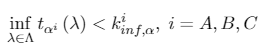
The null hypothesis that ZA pose for the three models is:
 [A.1]
[A.1]Thus, it is considered that under H0 the series is integrated without structural changes. Then, the selection of λ is the result of search for a dummy3 that achieves a stationary representation of yt. This means that the alternative hypothesis implies stationarity with a single break. The objective is then to estimate the break (the dummy) that most ponder the alternative of stationarity.
λ is chosen to minimize the one tail t-statistic, testing that αi = 1 for i = A,B,C, since small values of the statistic denote rejection of the null. In other terms,
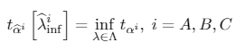 [A.2]
[A.2]where Λ (0,1).
As now the null is specified as in 5. Then, the equations for return in ZA unit root test are:
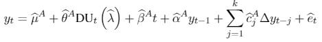 [A.3]
[A.3]
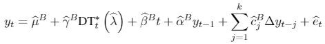 [A.4]
[A.4]
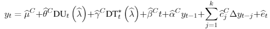 [A.5]
[A.5]where DUt if , 0 otherwise; if t>T , 0 in any other case. is the estimated break point after the mentioned procedure.
For each λ, the number of k extra lags, were determined using the Perron’s procedure4. Then, the t-statistic is computed. The minimum t obtained on T −2 regressions indicate then the estimated break date.
Once the selection of λ is no longer exogenous through the estimation method, ZA can no longer use the critical values computed by Perron. Now H0 is rejected if:
 [A.6]
[A.6]with as the critical size α (toward the left tail of the distribution of the statistic) of the asymptotic distribution of . Here, ZA claim that, by definition, these critical values are at least as large as those obtained under an exogenous λ. From this perspective then, the unit root test of Perron would be biased to reject the null hypothesis.
A.1.2 Kim - Perron (KP)
Regarding the test of Zivot and Andrews, Kim and Perron (2009) mentions:
“Zivot and Andrews assumed that if a break occurs, it does so only under the alternative hypothesis of stationarity. This is undesirable since a) it imposes an asymmetric treatment when allowing for a break, so that the test may reject when the noise is integrated but the trend is changing; b) if a break is present, this information is not exploited to improve the power of the test.”
Given these two issues, KP propose a testing procedure that allows a structural break under both the null and the alternative, and when a structural break is present, the asymptotic distribution of the test is the same as the case with a known break in the series, thus allowing increased power while maintaining a proper size test.
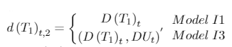
KP considers a univariate process yt generated by any of the three models of Additive Outliers (Additive Outliers, AO), or any of the two models of Innovative Outliers (Innovational Outliers, IO). For each model, the series is generated by the sum of a deterministic trend and an error term. The deterministic trend has a single break that occurs in a given period in the intercept, slope, or both, depending on the model.
The data generating processes (DGP) of the AO models are:
 [A. 7]
where ,
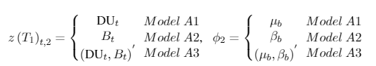
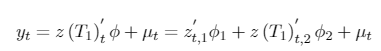
with DUt = Bt = 0 if t ≤ T1, and DUt = 1, Bt = t − T1 if t > T1. Here, T1 = λCT, with 0 < λC < 1, that denotes the true break (and λCthe true fraction that this break represents). Note that DUtand Bt depend on T1 and T but this dependence is omitted. The error {µt} is such that A(L)µt = B(L)εt where εt i.i.d , and A(L) and B(L) are polynomials L of order p + 1 and q, respectively. A(L) is factored as (1 − αL) (L) and is assumed that (L) and B(L) have roots strictly outside the unit circle. The null and alternative hypothesis are H0 : α = 1 and H1 : |α| < 1, respectively. The specified ARMA model can be relaxed to allow even more general processes but uses these specifications to facilitate the presentation of the test. The DGP of the innovational outlier (IO) models under the null hypothesis are given by:
 [A.8]
[A.8]where
and D(T1)t = 1 if t = T1 + 1 and 0 otherwise.
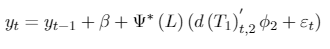
Under the alternative hypothesis:
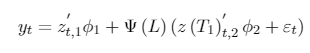 [A.9]
[A.9]where
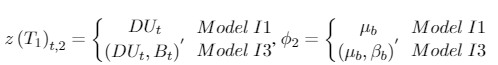
with Ψ∗ (L) and Ψ(L) such that Ψ∗ (L) = A∗ (L)−1 B (L) and (1 − αL)−1 Ψ∗ (L) = Ψ(L).
The authors point out at this point that the models A1, A2, A3 (with µb = c + βbT1), I1 and I3 (with µb = c + βbT1) are the same as in Perron (1989), except that the structural change is unknown (i.e. the potential date of the break is unknown).
Here, it should be noted that what is done is to test first a similar test to the one implemented in Perron (1989), but instead of using the actual date break, using an estimate of the same. The Perron procedure tests the unit root hypothesis on the sum of the autoregressive coefficients of the regression on the series that was previously removed the trend (for both AO and IO models). The result of this test is that . So, using an estimation of λ, the desirable condition is that . If this result holds, then one can use the critical values for the case where λ is known.
To estimate the break, Kim and Perron (2009) focus on the method to minimize SSR. Then KP’s work shows that the condition mentioned is true under certain assumptions, depending on the case of DGP in question. To fulfill this condition, as mentioned at the beginning of this subsection, the size improvement to be working with the distribution as if the breakdown was known rather than unknown.
A.2 Tables
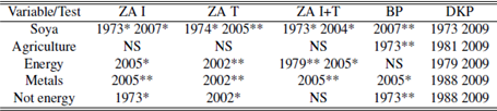
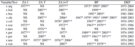
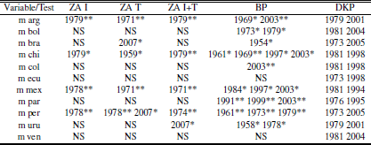
Perron test; *,** significance at 5% and 1% respectively; NS: No significative breaks.
Notes
Author notes
San Andrés 800-, Tel.: 54-(0291)-4595138, Bahía Blanca (8000)