
APPLICATION OF FACTOR ANALYSIS IN PRODUCTIVITY INDICATORS OF IDENTIFICATION IN A COMPANY OF RED CERAMIC INDUSTRY
Revista Produção e Desenvolvimento
Centro Federal de Educação Tecnológica Celso Suckow da Fonseca, Brasil
ISSN-e: 2446-9580
Periodicity: Frecuencia continua
vol. 4, no. 2, 2018
Received: 20 October 2017
Accepted: 28 April 2018
Published: 28 April 2019
Abstract: This study aims to identify which productivity indicators are most relevant, in other words, great explanatory power in performance evaluation in a company of red ceramic department. It is intended from this work, verify if the indicators used by the company are really the most relevant to evaluate the performance of the production process of ceramic blocks. This is a quantitative, exploratory, ex post facto and documentary study. For the assessment of the data on indicators currently measured and evaluated by the company, Factor Analysis (FA) was used. The analysis was done with 10 indicators of productivity, with a sample of 261 observations per indicator. Had it as an aid in modeling, the IBM SPSS version 23.0 software. In the end of analysis, culminating with only 5 variables, these were represented by two factors: production yield (factor 1 with 58.71% of explaining the variability of the model, represented by three indicators) and processing yield (factor 2 with 26 62% of explanation, represented by two indicators). In total, 85.33% of the variability of the model.
Keywords: Productivity indicators, Factor analysis, Multivariate analysis, Red pottery.
INTRODUCTION
Productivity is an important issue for any level of an organization. It can be said that the ultimate goal of every manager is to increase the productivity of the organizational unit under his responsibility, without, however, neglecting quality. Increases in productivity enable increases in customer satisfaction rates; waste reduction; reduction of material stocks; reduction in sales prices; reduction in delivery times; better use of human resources; increase in profits; safety at work; and higher wages ( Martins & Laugeni, 2005).
The concept of productivity was introduced in organizations in order to evaluate and improve performance. Initially, productivity was calculated by the ratio between the output of production and the number of employees, a formula that propagated over a long period, through which the increase in production per employee was sought. Other alternatives to measure productivity have emerged over time, relating the output of production to the use of resources such as energy, raw materials, inputs, among others ( Singh et al., 2000; Ukko et al., 2007; King et al., 2014).
Linked to this theme, productivity indicators have been used for a long time by people, organizations and nations to measure and monitor their own performance ( King et al., 2014). Currently, to quantify the productivity in a company, one must compare what was generated with what was used of resources to produce a given good and/or service. In this sense, productivity indicators are very important, since they allow an accurate evaluation of the effort employed to generate the products and services. It is a relation between two different units of measurement: one to quantify the resources used and another to quantify the outputs produced.
Productivity has always been a great indicator of the success or failure of companies, and is not different from those of the red ceramic sector, which are characterized by the production of blocks of reddish color, such as bricks, blocks, roof tiles, ducts, slabs, ornamental vases, aggregates of expanded clay, among others. The productive process in these companies consists of two stages: the primary one, which involves exploration and export of the raw material; and the secondary or processing, which consists of the elaboration of the final product, the productive process itself.
The productivity indicators measured in the red ceramic sector are defined by the managers of the companies without support of scientific criteria, that is to say, without consulting the specialized literature. With many indicators available, the analyst needs to check the importance of each one of them and point out which are the main ones ( Soares, 2006). According to Iudícibus (1998), it is much more useful to calculate a selected number of indexes than to calculate tens and tens of indexes without correlation with each other, without comparisons and also try to give a focus and a meaning of these indexes.
Thus, this study aims to identify, through a Factorial Analysis (FA), which productivity indicators are more relevant, that is, greater explanatory power in the performance evaluation in a company of the red ceramic sector located in the county of Rio Tinto (PB), Brazil.
In addition, this study seeks to assist companies in the red ceramic sector in the analysis and selection of productivity indicators that will be used in performance evaluation. The theoretical contribution of the study is in the perception of the still small amount of work in the red ceramic sector, mainly focusing on productivity and productivity indicators.
THEORETICAL REFERENCE
Productivity
The success of a business do not depends only on a quality product but also on the continuous increase in productivity to remain competitive, since by improving productivity an organization can benefit from cost and quality advantages compared to its competitors ( Snyman, & Smallwood, 2017). Productivity is considered a key factor in measuring the performance of a company's manufacturing system ( Rawat et al., 2018). According to Martins & Laugeni (2005), the term productivity was first used officially in an article by the French economist Quesnay in 1766. In 1883, another French economist, Littre, used the term with sense of "capacity to produce". At the beginning of the twentieth century, the term assumed the meaning of the relation between what was produced (output) and the resources used to produce it (input).
In 1950, the European Economic Community presented a formal definition of productivity as "the quotient obtained by the division of production by one of the factors of production", thus allowing to speak in productivity of capital, raw materials, labor, among others ( Martins & Laugeni, 2005).
For Rodrigues (2004), the productivity is related to the production of goods or services, and is represented by the ratio of what is necessary to accomplish the production by the final result. Gronroos and Ojasalo (2004) complement the aforementioned author by defining productivity as a measure of how input resources are used and transformed into value for customers. While Chen & Liaw (2001) and Huang et al. (2003) treat productivity as an indicator of efficiency.
Generally, the productivity of a productive system can be defined as the relation between what is generated by the system (its products or outputs) and what enters that system (its incomings or inputs) in a certain period of time. It implies in the establishment of two basic categories of measures: static productivity, originating from the division of the measures of the outputs by the measures of the inputs, in a given period of time; and dynamic productivity, defined as the relationship between static productivity measures at different periods, reflecting productivity variation from one period to another ( Torres Júnior & Lopes, 2013).
The definition that will guide this study is the one most used today in the specialized literature, that is, productivity is a quotient obtained in the division of a product by one of its elements of production, namely: raw material, workmanship, machinery and equipment, electricity, water, time spent, idle time, rework, etc.
Performance Indicators
Given the current competition in the market, companies need to monitor their practices and results to ensure competitiveness. To survive these challenges and compete successfully, organizations need to monitor processes through Performance Indicators ( Silva & Borsato, 2017). Performance Indicators are key managerial tools for decision making in organizations ( Gunasekaran et al., 2015) and important for monitoring the performance of a productive sector ( Lindberg et al., 2015). They allow to gather knowledge and explore the best way to achieve the objectives of an organization ( Badawy et al., 2016).
According to Martins & Laugeni (2005), performance indicators are indexes to measure a certain quantity of a manufacturing or administrative process, to determine if the process is within the acceptable parameters. If not, management and operational actions are determined that will lead the process to performance. For the authors, the main indicators are Productivity and Quality of Service. Soares (2006) says that a performance indicator is a measure such as percentage, index, quotient, rate or other comparison, which is monitored at intervals and compared to one or more criteria. According to Tadachi & Flores (2005), indicators are quantifiable forms of representation of the characteristics of products and processes. They are used by the organization to control and improve the quality and performance of its products and processes over time.
Nova (2002) comments that performance indicators are used to quantitatively measure performance in a company and uses as benchmarks numerical indices such as percentages, quotients, amounts, multipliers. The author lists characteristics of the performance indicators that should be observed:
Objectivity: subjective indicators make it difficult to measure, which justifies the preference for quantitative data;
Measurability: Indicators should be measurable, in the sense that their quantification is possible on a given scale of values;
Comprehensibility: indicators are used to inform performance, therefore, measures that have meaning for managers should be used;
Comparability: indicators should be comparable between periods for the same entity and between entities or other companies within the same evaluation sector;
Cost: the evaluation should always consider a cost/benefit analysis, the information generated must have its utility at the cost of obtaining it.
Batista (1999) typifies the indicators as follows:
Strategic indicators: inform how the organization is in the direction of achieving its vision, reflecting performance in relation to critical success factors;
Indicators of productivity (efficiency): measure the proportion of resources consumed in relation to the outputs of the processes;
Quality indicators (effectiveness): focus on measures of customer satisfaction and the characteristics of products or services;
Indicators of effectiveness (impact): focus on the consequences of products or services;
Capacity indicators: measure the responsiveness of a process through the relationship between the outputs produced per unit of time.
For Rodrigues (2004), the most frequently used performance indicators are productivity, capacity, flexibility, speed and reliability. Given the focus of this study, the subsequent topic will discuss productivity indicators.
Productivity Indicators
At the end of 19th century, the works of Frederick W. Taylor, considered the father of the Scientific Administration appeared in the United States. With his works, the systematization of the concept of productivity arises, that is, the incessant search for better working methods and production processes, with the aim of achieving improved productivity at the lowest possible cost. This demand is still the central theme in all companies, changing only the techniques used. The analysis of the relationship between output and input allows us to quantify productivity, which has always been a great indicator of companies? success or failure ( Martins & Laugeni, 2005). According to Martins & Laugeni (2005), the productivity of a company can be evaluated by the following indicators:
Total Productivity (TP): the relationship between the output measured between two instants (i, j), at the prices of the initial instant and the measure of the input consumed between the two instants (i, j), at the prices of the initial instant ;
Partial productivity of labor (PP) or manpower: the ratio between total output in the period, at constant prices, and labor input in the same period, at constant prices;
Partial capital productivity (PP): the ratio between total output in the period, at constant prices, and capital input in the same period, at a constant rate of return;
Partial material productivity (PP): the ratio between the total output in the period, at constant prices, and the input of the intermediate materials purchased in the period, at constant prices.
Torres Júnior & Lopes (2013) say that depending on the number of inputs considered, the following productivity indicators can be obtained:
Partial productivity: when considering only one of the inputs (labor, capital, energy, raw materials, etc ...);
Total factor productivity: when capital and labor inputs are considered simultaneously, they are weighted according to certain rules to give a single measure of inputs;
Total Productivity: when considering all inputs.
Factorial Analysis
Factorial Analysis (FA) is a generic name given to a class of multivariate statistical methods whose main purpose is to define the underlying structure in a data matrix. It addresses the problem of analyzing the structure of interrelationships (correlations) between a large number of variables, defining a set of latent dimensions, called factors ( Hair et al., 2009). Its purpose is to unveil existing structures, but they are not directly observable, so Furtado and Furtado (2017) comment that FA has as one of its objectives to intend to describe a set of original variables, by creating a smaller number of dimensions or factors.
Tian et al. (2018) define factorial analysis as a multivariate statistical analysis method that studies the relationship between the correlation matrix of the sample and the number of variables or samples that have a certain relation to the number of unobservable factors (also known as factor main).
FA assumes that high correlations between variables generate clusters that configure the factors, in other words, the existence of the factor explains the correlation in a certain group of variables. Thus, after creating factors, FA ends up simplifying complex relationship structures, allowing a better understanding of the data structure.
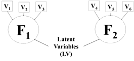
According to Hair et al. (2009), with FA, the researcher can first identify the separate dimensions of the structure and then determine the degree to which each variable is explained by each dimension; the dimensions and the explanation of each variable, the summary and the reduction of the data can be obtained. For the authors, in summarizing the data, the Factor Analysis obtains latent dimensions that, when interpreted and understood, describe the data in a much smaller number than the original individual variables. Figure 1 graphically illustrates the simplification of the phenomenon by the use of FA.
FA assumes that the correlation between variables arises because these variables share or are related by the same factor ( Bezerra, 2009). In this sense, the author comments that the main objective of FA is to identify factors not directly observable, based on the correlation between a set of variables, which are observable and measurable.
The most commonly used method of FA is the Exploratory Factor Analysis (EFA), which is characterized by the fact that it does not require the researcher to know the relationship between the variables prior to their use ( Bezerra, 2009). In this type of FA, the researcher is not sure that the variables have a relationship structure. He/she analyzes, understands and identifies a relationship structure between the variables from the FA result. In the present study, we chose to use this modality of multivariate analysis.
Hair et al. (2009) states that under the exploratory perspective, factorial analytical techniques consider what the data offer and do not establish restrictions on the estimation of components or on the number of components to be extracted.
According to Bezerra (2009), prior to performing FA, the researcher must make some choices that will be influenced by the type of research to be performed, namely: the method of extracting the factors to be used, the type of analysis to be carried out; how the choice of factors will be made; and how to increase the explanatory power of FA. Table 1 summarizes these choices, listing and describing possible alternatives.
| Choice | Alternatives | Description |
| 1. Method of extracting the factors to be used | Main Components Analysis (PCA) | The total variance in the data is taken into account. It is recommended when the researcher is interested in determining factors that contain the highest possible explanation of the variance and also for the treatment of the data for use in other statistical techniques that are detrimental to the correlation between the analyzed variables. |
| Common Factorial Analysis | Factors are estimated based only on the common variance. It is indicated for researchers whose main objective is to analyze the underlying structures of relationship between variables. It should be used when the researcher has a good understanding of the variables under analysis, so he will be able to make a greater number of inferences about relationships created by FA. | |
| 2. Type of analysis to be performed | R-mode factor analysis | Used when trying to identify underlying structures capable of being perceived only by building relationships between several variables. |
| Q-mode factor analysis | Used when you are interested in creating clusters of cases. | |
| There are other types of analysis that can be used with FA, but less usual, such as: O-mode factor analysis, T-mode factor analysis and S-mode factor analysis. | ||
| 3. How will the choice of factors be made | Autovalue Criterion | The eigenvalue corresponds to how much the factor can explain the variance, that is, how much of the total variance of the data can be associated with the factor. Only factors with eigenvalues above 1.0 are considered. Also called latent root criterion or Kaiser criterion (Kaiser test). |
| Slope chart criterion or scree plot | It follows the reasoning that a large portion of variance will be explained by the first factors and that between them there will always be a significant difference. When this difference becomes small (curve smoothing), this point determines the number of factors to consider. | |
| Percentage of variance explained | The percentage of explanation of the variance is taken into account. The number of factors to be extracted is the one that explains a percentage of variance considered adequate by the researcher. | |
| 4. How to Increase the Explaining Power of FA | Rotation of Factors | An FA will be more or less useful according to its ability to produce factors that can be translated. However, there are cases where more than one of the factors explains the behavior of one of the variables. In these cases, solutions must be sought that explain the same degree of total variance, but that generate better results in relation to their interpretation, which can be done through the rotation of the factors. There are several methods of rotation, such as: (1) Varimax, orthogonal rotation type, the most used; (2) Quartimax; (3) Equimax; (4) Direct Oblimin; (5) Promax. |
| Factorial loads | FA parameters that relate the factors to the variables, making possible the interpretation of the factors. They represent the correlation between the factor and the study variables. | |
| Communalities | They represent the percentage of explanation that the variable obtained by the FA, that is, how all the factors together are able to explain a variable. The closer to number one, the greater the explanatory power of the factors. | |
As to the percentage of variance explained, Hair et al. (2009) defines that in the natural sciences, the procedure of obtaining factors should not be stopped until the factors extracted explain at least 95% of the variance or until the last factor explains only a small portion, less than 5%. However, the authors comment that in social sciences, where information is not as accurate as in the natural sciences, at least 60% of the total variance can already be considered satisfactory.
According to Bezerra(2009) and Sun et al. (2017), the steps to be followed in developing a FA are:
Calculation of the correlation matrix: the degree of relationship between the variables and the convenience of the application of FA is evaluated;
Extraction of the factors: determination of the method for calculating the factors and definition of the number of factors to be extracted; trying to find out how much the model is appropriate;
Rotation of factors: we seek greater capacity to interpret the factors;
Calculation of scores: results in scores that can be used in other analyzes.
In addition to these points, care should be taken regarding the sample size. Pestana & Gageiro (2014) indicate 5 observations per variable. Stevens (2009) recommends 5 to 20 observations per variable. Hair et al. (2009) argues that it is necessary 20 cases per variable. Regarding the correlation matrix, the authors emphasize that if a visual inspection does not reveal a substantial number of correlations greater than 0.30, then Factorial Analysis is probably inappropriate. In the correlation matrix, the values of the test of significance (p-test) should be close to zero to obtain a good FA. Table 2 describes, according to Bezerra (2009) and Hair et al. (2009), the tests used to evaluate if the original data of the research make FA satisfactory:
| Test | Bezerra (2009) | Hair et al. (2009) |
| Kaiser-Meyer-Olkin Test - KMO (Measure of Sampling Adequacy - MSA) | Indicates the degree of explanation of the data from the factors found in FA. If the MSA indicates a degree of explanation of less than 0.5 means that the factors can not satisfactorily describe the variations of the original data. | The MSA index ranges from 0 to 1, reaching 1 when each variable is perfectly predicted without errors by the other variables. The measure can be interpreted with the following guidelines: ? 0.80 (admirable); ? 0.70 and below 0.80 (median); ? 0.60 and below 0.70 (mediocre); ?0.50 and below 0.60 (poor); <0.50 (unacceptable). |
| Bartlett's Sphericity Test | Indicates if there is a sufficient relationship between the variables for the application of FA. It is recommended that the value of the test of significance does not exceed 0.05, otherwise it is probable that the correlation of the variables is too small, which prevents the application of the FA. | Statistical test for the presence of correlations between variables provides the statistical probability that the correlation matrix has significant correlations between at least some of the variables. |
| Matrix of correlation anti-image | Indicates the explanatory power of the factors in each of the analyzed variables. Values on the main diagonal of the matrix less than 0.50 are considered too small for analysis, and in these cases indicate variables that can be removed from the analysis. | It consists of the negative value of the partial correlation. Partial correlations or larger anti-image correlations are indicative of a matrix of data that may not be suitable for factor analysis. |
Table 2 presented the tests used to evaluate the feasibility of a Factor Analysis satisfactorily. However, once FA is performed, the reliability of its factorial structure should be ascertained.
According to Sijtsma (2009), one of the main criteria of consistency presented in the literature is the calculation of the internal consistency index, through Cronbach's Alpha, criterion presented by Lee Cronbach, in 1951. Pereira et al. (2018) consider the Cronbach's alpha coefficient to be one of the main questionnaire reliability estimators. Taber (2017) commented that this alpha is commonly reported for the development of scales designed to measure attitudes and other affective constructs. Hora et al. (2010) define the Conbach Alfa as a way of estimating the reliability of a questionnaire applied in a research; the alpha presents the function of measuring the correlation between the answers of a questionnaire by analyzing the profile of the answers given by the respondents, treating it as a mean correlation between questions.
According to Vaske et al.(2017), the Conbach's alpha measures the extent to which item responses (responses to survey questions) are correlated with each other, so it can be said that ? estimates the proportion of variance that is systematic or consistent in a set of research responses. Maroco & Garcia-Marques (2006) comments that Cronbach's alpha index varies on a scale of 0 to 1, where the closer to one, the greater the reliability of the analysis. For the interpretation of the alpha, there is no consensus among the authors about the reliability of a questionnaire obtained from the value of this coefficient. Works as with Urdan?s (2001), Oviedo & Campo-Arias? (2005) and Milan & Trez?s (2005) recommend at least 0.70 Cronbach's alpha index. George & Mallery (2003) suggest more detailed values ??for interpretation, such as: excellent (Alpha above 0.90); good (0.80 <Alpha ? 0.90); acceptable (0.70 <Alpha ? 0.80), questionable when it is below 0.6 and unacceptable when below 0.50. Simões & Pellegrinotti (2017) and Passos et al. (2017) indicate an alpha from 0.70 as satisfactory. Moreover, Azevedo-Santos et al. (2017) define an alpha between 0.70 and 0.80 as acceptable and above 0.80 as good.
METHODOLOGY
This study is a research of a quantitative nature, since, according to Bezerra & Corrar (2006) and Wagner et al. (2017), a statistical method is used, based on the survey of past occurrences and the extrapolation of the knowledge acquired for future occurrences, using statistical techniques. It is considered exploratory research, since the attributes of the variables used are numerical and it is intended to increase the existing knowledge about the use of multivariate statistical analysis tools in the identification of productivity indicators in a company of the red ceramic sector. In addition, it may be considered an ex post facto research, since it is not possible the researcher's interference in the study variables.
The research was carried out in a company of the red ceramic sector, located in the county of Rio Tinto (PB). The products manufactured by the company are classified in the following categories: Bricks /Sealing Blocks; Structural brickwork; Slabs / Building Blocks; Troughs/Gutters; and Special Blocks. Its production system is characterized by high degree of uniformity, large-scale production, highly standardized products, a sequence of pre-established and very well-defined operations.
The research?s primary data were extracted from daily records of the company's production, so the research is documentary as to the technical procedures used. Data collection was done by the Manager of the manufacturing unit, who was directly responsible for the measurement and evaluation of productivity indicators used by the company. Table 3 presents and describes the productivity indicators of the company, which were transformed into study variables, for later analysis.
| Study variable | Productivity Indicator | Description |
| X01 | Parts Produced (un.) | Quantity, in units, of ceramic blocks produced per work shift, withdrawing products with malfunctions. |
| X02 | Produced kilos (kg) | Weight, in kilograms, of the total number of ceramic blocks produced per work shift, with the removal of defective products. |
| X03 | Processed Meters (m.) | Length, in meters, of the total number of ceramic blocks produced per shift, including products with breakdowns. |
| X04 | Processed Parts (un.) | Quantity, in units, of ceramic blocks produced per shift, including products with breakdowns. |
| X05 | Processed Kilos (kg) | Weight, in kilograms, of total ceramic blocks produced per shift, including products with breakdowns. |
| X06 | Yield of Parts | Ratio between the quantity produced and the quantity processed. |
| X07 | Useful time (min.) | Time, in minutes, per work shift, effectively used in the production of ceramic blocks. |
| X08 | Time worked (min.) | Time, in minutes, per work shift, spent in production, including scheduled and non-scheduled intermissions. |
| X09 | Yield Time | Ratio between working time and time of actual work. |
| X10 | Processed Kilos (kg) / Useful Time (min) | Ratio between kilograms of material processed and time (kg / min). |
For each productivity indicator, there are 261 observations. The observations represent approximately 130 working days, between the months of September and December of the year 2015. The factorial analysis was complemented with the use of the software IBM SPSS version 23.0.
ANALYSIS AND DISCUSSION OF RESULTS
Table 1 presents descriptive statistics of the indicators. As there are variables with different units of measure, we chose to calculate the coefficient of variation - CV (ratio between the standard deviation and the mean). Therefore, the variable Yield Time - X09 presented greater variability (541.7%) and Processed Kilos - X10, lower (62.8%). Sample of 261 observations is compatible with the minimum recommendation of Hair et al. (2009) of at least 20 cases per variable.
| X10 | 558.45 | 889.67 | 62.8% |
Attempt with all indicators
According to Table 2, the Kaiser-Meyer-Olkin test (Measurement of Sampling Adequacy - MSA) resulted in 0.655, which is an acceptable value for the analysis, according to Hair et al. (2009). Thus, there are indications that the factors can reasonably describe the variations of the original data, that is, the performance of the factor analysis is satisfactory due to the correlation between the variables. The Barlett's sphericity test presented significance at 5% (p-value = 0.000), that is, there is an indication of the possibility of application of FA in the variables analyzed.
| Kaiser-Meyer-Olkin Test (KMO) | 0.655 |
| Bartlett's Sphericity Test | 3504.86 |
| Degrees of freedom | 45 |
| p-value | 0.000 |
The anti-image correlation matrix ( Table 3) presents the explanatory power of the factors in each variable. The main diagonal indicates the MSA (Measure of Sampling Adequacy). It is observed that with a single exception, all variables are above 0.50, which is a desirable result for the model, since these values ??validate the use of all the remaining indicators in the FA. The only exception was the case of the variable Yield Time (X09), because its MSA is below 0.5; there are indications that it may be withdrawn from the analysis.
| X01 | X02 | X06 | X08 | X03 | X04 | X05 | X07 | X09 | X10 | |
| X01 | 0.572ª | |||||||||
| X02 | -0.826 | 0.620ª | ||||||||
| X06 | 0.137 | -0.419 | 0.717ª | |||||||
| X08 | -0.061 | -0.341 | 0.087 | 0.840ª | ||||||
| X03 | 0.193 | 0.023 | -0.052 | -0.322 | 0.781ª | |||||
| X04 | -0.835 | 0.750 | -0.114 | -0.032 | 0.296 | 0.516ª | ||||
| X05 | 0.562 | -0.659 | 0.271 | 0.141 | -0.625 | -0.884 | 0.591ª | |||
| X07 | 0.059 | -0.118 | 0.195 | -0.319 | -0.091 | -0.091 | 0.098 | 0.867ª | ||
| X09 | -0.024 | -0.054 | -0.233 | 0.443 | -0.110 | 0.022 | -0.020 | -0.456 | 0.469ª | |
| X10 | -0.317 | 0.286 | 0.090 | 0.193 | -0.002 | 0.359 | -0.394 | 0.098 | 0.126 | 0.624ª |
Table 3 shows a low MSA for the variable Yield Time (X09). However, even though it shows little relation with the factors, according to Table 4, this presented commonality of 0.771, that is, this value represents the power of explanation considering all the factors obtained.

Figure 2 graphically represents the percentage of variation explained by the component in the ordinates and the eigenvalues, in descending order. In this way, it is possible to graphically analyze the dispersion of the number of factors until the individual variance curve of each factor becomes horizontal or abruptly falls. A fall from the fourth factor is observed, and there are indications of using three factors in the model.
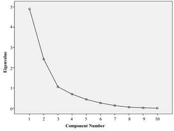
Table 5 illustrates that, through three factors, the model explains almost 84% of the variance of the original data (83.799%), thus corroborating the indications in Figure 2.

After analyzing the degree of explanation of the productivity indicators model, Table 6 identifies which indicators are part of each of the factors. The Component Matrix allows you to check which factor best explains the indicators. However, this matrix causes doubts about the composition of each factor in relation to the data, since there are very close explanatory values ??in some cases (note that factor loads below 0.30 were excluded); in these cases, Tian et al. (2018) and Rocha et al. (2018) recommend the verification of the values ??after the application of factor rotation by the Varimax criterion.

Table 7 shows the matrix after factor rotation, in which there are still doubts regarding the selection of the indicators. Since, according to Hair et al. (2009), after identifying variables with high factor loads above 0.40 in both components, the authors argue that the same variable can not contribute to the construction of different factors. Thus, Andersen et al. (2017) suggest to adopt 0.40 as the acceptable limit of the contribution of the variable in the creation of the factor, in order to avoid the problem of indetermination, the relation between variables and factors. However, even when rotating, four variables violated this assumption (X03, X04, X05 and X07). Thus, we opted for the exclusion of the smallest number of variables, selecting Table 6, indicating X01, X04 and X05 for FA removal.

Attempt with 7 indicators
After extracting the three indicators (X01, X04 and X05), according to Table 8, an improvement in the explanatory power of the model was detected. The KMO test was 0.677 (higher than the previous 0.655 trial of Table 2). The sphericity test remained significant at 5%. The Anti-Image Matrix that displays the individual MSA values ??( Table 8) detected an indicator less than 0.50 (X09).
| X02 | X06 | X08 | X03 | X07 | X09 | X10 | |
| X02 | 0.735ª | ||||||
| X06 | -0.327 | 0.615ª | |||||
| X08 | -0.736 | -0.009 | 0.655ª | ||||
| X03 | -0.061 | 0.298 | -0.318 | 0.728ª | |||
| X07 | -0.120 | 0.217 | -0.343 | -0.078 | 0.813ª | ||
| X09 | -0.177 | -0.277 | 0.457 | -0.268 | -0.456 | 0.402ª | |
| X10 | -0.196 | 0.385 | 0.281 | -0.435 | 0.152 | 0.128 | 0.559ª |
Table 9 presented the same indicator with commonality 0.250. For these reasons, this variable was excluded from the study and a new factorial analysis will be performed with 6 indicators.

Attempt with 6 indicators
The new FA, now with 6 indicators, showed the KMO test equal to 0.724 (higher than the analysis of topic 4.2). The sphericity test remained significant at 5%. The Anti-Image Matrix ( Table 10) presented all the indicators with MSA values ??above 0.50. Table 11 presents the commonalities. It is observed in this case that all are above 0.77.
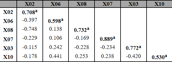
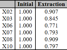
Table 12 illustrates, by means of two factors, an explanation of 83.71% of total variability, a result similar to Table 5, but with four variables less. It is observed the possibility of representing the same percentage with fewer variables.

The Component Matrix is ??presented in Part I of Table 13. Note that an indicator (Processed Meters - X03) has factorial loads close to both factors. In this way, Part II illustrates the rotated components. Again X03 presented high load, for this reason, it was chosen for its withdrawal and realized again an FA, now with 5 indicators.

Attempt with 5 indicators
With a new FA performed, now with 5 indicators, the KMO test resulted in 0.655 (lower than the attempt of topic 4.3). The sphericity test remained significant at 5%. Table 14 shows the Anti-Image Correlation Matrix with all individual MSAs greater than 0.50. The commonalities are illustrated in Table 15. It is observed that all are above 0.79. This is a very satisfactory result.
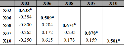
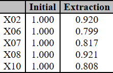
Table 16 presents, through two factors, a total explanation of the original data variability of 85.328% (above that obtained in the model of topic 4.3 with 6 indicators). Thus, with 5 variables, we obtained the highest percentage of explanation of the total variance of the model. Although the second factor of FA is extremely relevant for the analysis, Szabó & Dobróka (2018) consider the first most important factor to present a higher percentage of explanation of the total variance.

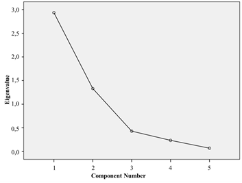
Based on the Scree Plot of Figure 3, a fall from the 3rd factor is observed, corroborating the use of only two factors, a fact already seen in Table 16.
The Component Matrix is ??presented in Part I of Table 17. Note two indicators (Processed Kilos/Useful Time - X10 and Yield Parts - X06) with factorial loads on both factors. By analyzing the rotated factors, Part II detects all the indicators with factorial loads in only one factor.

The matrix, after factor rotation (Part II of Table 17), allows a more accurate classification of the indicators in each of the two factors. Therefore, it can be concluded that FACTOR 1 is composed of Kilos Produced (X02); Useful time (X07) and Time worked (X08). FACTOR 2 is composed of Processed Kilos/Useful Time (X10) and Yield Parts (X06).
From this selection of factors, it was possible to name the first factor as the yield of production (F1), the second factor interpreted as the yield of processing (F2). In order to verify the internal consistency of the factors, Cronbach's alpha was used. Factor 1 had an Alpha of 0.935 and Factor 2 had an Alpha of 0.752. This means that the factors presented good internal consistency, since they were higher than 0.7.
Consideration on productivity indicators excluded from the FA
The study began with 10 indicators of productivity, however, in the end represented by two factors, culminated in only 5. However, it is possible to observe that all the indicators that were excluded from the analysis, they underwent several tests to verify the possibility of creating clusters between these variables that could result in other factors that, isolated from the three factors initially identified, would represent the evaluation model of productivity indicators.
However, the results of these tests were not sufficient to maintain these indicators in the factor analysis. In all attempts to work with the eliminated factors, in none of the analyzes, the KMO value exceeded 0.56. Moreover, in most attempts, the model did not fit the data; and even rotating the component matrix, there was still a variable with a high factor load in more than one factor.
Another criterion also used, besides the percentage of total variance explained by the minimum model of 70%, was the calculation of Cronbach's alpha, which in all the attempts, it was inferior to 0.5. Therefore, due to these reasons and those presented previously, the excluded variables did not become part of the model for evaluating productivity indicators.
FINAL CONSIDERATIONS
This study aimed to identify which productivity indicators are of greater relevance in the performance evaluation of a company in the red ceramic sector. The application of FA allowed to summarize and identify the indicators of greater explanatory power, considering the composition of the factors obtained.
The factors found by Factor Analysis demonstrate the main concerns that the manager of the company of the red ceramic sector should have when it seeks to maximize productivity through indicators.
Factor 1 suggests greater attention to productivity yield, accounting for 52.76% of the total variance explained in the model. This factor is represented by the indicators:
Kilograms Produced: Weight, in kilograms, of the total number of ceramic blocks produced per work shift, removing the damaged products. This way, the greater the quantity of kilos produced, the better for the company, since the quality control is strict, and therefore, represents high production of material.
Time worked: Time, in minutes, per work shift, spent in production, including program stops (SETUP time) and unscheduled. A high uptime is not necessarily a positive time, since it is possible that there are many stops in the production process, thus reducing productivity.
Useful time: Time, in minutes, per work shift, effectively used in the production of the ceramic blocks. The higher this time the better, once this period has already been discounted the time of non-productivity.
Factor 2 presented a lower level of explanation than Factor 1. Representing 32.56% of total variability. This factor consists of two indicators:
Processed Kilograms/Time: Ratio between kilograms of material processed and time measured in minutes. In this way, you can analyze how much is processed in ceramic material per minute. Therefore, the higher this value, the better, after all, it is a sign that the company is showing a high level of production.
Yield Piece: Ratio between the quantity of parts produced and the quantity processed. That ratio the closer to one, the better. For example, if this quotient was exactly one, it is a sign that the productive process had very high productivity, after all, all the pieces produced were processed, so apparently there was no wastage or rework of the processes.
Therefore, the present study tends to assist companies in the red ceramic industry in the analysis and selection of productivity indicators that will be used in the evaluation of performance, through the application of a statistical tool. It is recommended that studies in this area be carried out in other production sectors, since the definition of productivity indicators varies according to the nature of the companies, be they manufacturing or services.

REFERENCES
ANDERSEN, C.M.; PEDERSEN, A.F.; CARLSEN, A.H.; OLESEN, F.; VEDSTED, P. Data quality and factor analysis of the Danish version of the Relationship Scale Questionnaire. PLoS ONE, v.12, n.5, 2017.
AZEVEDO-SANTOS, I.F.; ALVES, I.G.N.; NETO, M.L.C.; BADAUÊ-PASSOS, D.; SANTANA-FILHO, V.J.; SANTANA, J.M. Validation of the Brazilian version of Behavioral Pain Scale in adult sedated and mechanically ventilated patients. Brazilian Journal of Anesthesiology, v.67, n.3, p.271-277, 2017.
BADAWY, M.; EL-AZIZ, A. A. A.; IDRESS, A. M.; HEFNY, H.; HOSSAN, S. A survey on exploring key performance indicators. Future Computing and Informatics Journal, v. 1, n.1-2, p. 47-52, 2016.
BATISTA, F. F. Elaboração de indicadores de desempenho institucionais. São Paulo: Instituto Serzedelo Correa, 1999.
BEZERRA, F. A. Análise Fatorial. In: Corrar, L. J.; Paulo, E.; Dias Filho, J. M. (Coord.). Análise Multivariada: para os Cursos de Administração, Ciências Contábeis e Economia. São Paulo: Atlas, 2009.
BEZERRA, A. F. CORRAR, L. J. Utilização da análise fatorial na identificação dos principais indicadores para avaliação do desempenho financeiro: Uma aplicação nas empresas de seguros. Revista Contabilidade & Finanças, n. 42, p. 50?62, 2006.
CHEN, L. H.; LIAW, S. Y. Investigating resource utilization and product competence to improve production management: an empirical study. International Journal of Operations & Production Management, v. 21, n. 9, p. 1180-1194, 2001.
FURTADO, F.R.G.; FURTADO, R.C. Usando a análise fatorial para construir e validar um índice de inserção regional sustentável de usinas hidrelétricas. Revista Espaço Acadêmico, n.191, 2017.
GEORGE, D.; MALLERY, P. SPSS for Windows step by step: A simple guide and reference (4th ed.). 11.0 update. Boston: Allyn and Bacon, 2003.
GRONROOS, O. C.; OJASALO, K. Service productivity towards a conceptualization of the transformation of inputs into economic results in services. Journal of Business Research, v. 57, n. 43, p.414-423, 2004.
GUNASEKARAN, A., IRANI, Z.; CHOY, K.; FILIPPI, L.; PAPADOPOULOS, T. Performance measures and metrics in outsourcing decisions: A review for research and applications. International Journal of Production Economics, v. 161, p.153-166, 2015.
HAIR, J. F.; BLACK, W. C.; BABIN, B. J.; ANDERSON, R. E.; TATHAM, R. L. Análise Multivariada de Dados (6 ed.). Porto Alegre: Bookman, 2009.
HORA, H. R. M.; MONTEIRO, G. T. R.; ARICA, J. Confiabilidade em Questionários para Qualidade: Um Estudo com o Coeficiente Alfa de Cronbach. Produto & Produção, v. 11, n. 2, p. 85-103, 2010.
HUANG, S. H.; DISMUKES, J. P.; SHI, J.; SU, Q.; RAZZAK, M. A.; BODHALE, R.; Robinson, D. E. Manufacturing productivity improvement using effectiveness metrics and simulation analysis. International Journal of Production Research, v. 41, n. 3, p. 513-527, 2003.
IUDÍCIBUS, S. de. Contabilidade Gerencial (6 ed.). São Paulo: Atlas, 1998.
KING, N. C. O.; LIMA, E. P.; COSTA, S. E. G. Produtividade sistêmica: conceitos e aplicações. Production, v.24, n.1, p. 1-17, 2014.
LINDBERG, C-F.; TAN, S. T.; YAN, J. Y.; STARFELT, F. Key performance indicators improve industrial performance. Energy Procedia, v. 75, p.1785-1790, 2015.
MAROCO, J.; GARCIA-MARQUES, T. Qual a fiabilidade do alfa de Cronbach? Questões antigas e soluções modernas? Laboratório de Psicologia, v. 4, n. 1, p. 65-90, 2006.
MARTINS, P. G.; LAUGENI, F. P. Administração da Produção (2 ed.). São Paulo: Saraiva, 2005.
MILAN, G. S., TREZ, G. Pesquisa de satisfação: um modelo para planos de saúde. RAE Electron, v. 4, n. 2, p. 1-21, 2005.
NOVA, S. P. C. C. Utilização da análise por envoltório de dados (DEA) na análise de demonstrações contábeis. 2002. Tese. (Doutorado em Contabilidade e Auditoria). Utilização da análise por envoltório de dados (DEA) na análise de demonstrações contábeis, Universidade de São Paulo, São Paulo, 2002
OVIEDO, H. C., CAMPO-Arias, A. Aproximación al uso del coeficiente alfa de Cronbach, Revista Colombiana de Psiquiatría. v. 34, n. 4, p. 572-580, 2005.
PASSOS, M.H.P.; SILVA, H.A.; PITANGUI, A.C.R.; OLIVEIRA, V.M.A.; LIMA, A.S.; ARAÚJO, R.C. Reliability and validity of the Brazilian version of the Pittsburgh Sleep Quality Index in adolescents. Jornal de Pediatria, v.93, n.2, p. 200-206, 2017.
PEREIRA, L.W.; BERNARDI, J.R.; MATOS, S.; SILVA, C.H.; GOLDANI, MARCELO Z.; BOSA, VERA L. Cross?cultural adaptation and validation of the Karitane Parenting Confidence Scale of maternal confidence assessment for use in Brazil. Jornal de Pediatria, v.94, n.2, p.192-199, 2018.
PESTANA, M. H.; GAGEIRO, J. N. Análise de Dados para Ciências Sociais: A complementaridade do SPSS (6. ed.). Lisboa: Editora Silabo, 2014.
RAWAT, G. S.; GUPTA, A.; JUNEJA, C. Productivity Measurement of Manufacturing System. Materials Today: Proceedings, v. 5, n. 1, p. 1483?1489, 2018.
ROCHA, J.R.D.A.S.D.C.; MACHADO, J.C.; CARNEIRO, P.C.S. Multitrait index based on factor analysis and ideotype-design: proposal and application on elephant grass breeding for bioenergy. GCB Bioenergy. v.10, p.52-60, 2018.
RODRIGUES, M. V. Ações para a qualidade: GEIQ, gestão integrada para a qualidade: padrão seis sigma, classe mundial. Rio de Janeiro: Qualitymark, 2004.
SIJTSMA, K. On the use, the misuse, and the very limited usefulness of Cronbach?s Alfa. Psychometrika, v. 74, n. 1, p. 107-120, 2009.
SILVA, F. A.; BORSATO, M. Organizational Performance and Indicators: Trends and Opportunities. Procedia Manufacturing, v. 11, p. 1925-1932, 2017.
SIMÕES, R. & PELLEGRINOTTI, I.L. Preparation and body perception instrument validation in sports performance ? PECOPS. Revista Brasileira de Ciências do Esporte, v.39, n.4, p. 389-397, 2017.
SINGH, H.; MOTWANI, J.; KUMAR, A. A review and analysis of the state-of-the-art research on productivity measurement. Industrial Management and Data Systems, v. 100, n. 5, p. 234-241, 2000.
SNYMAN, T.; SMALLWOOD, J. Improving Productivity in the Business of Construction. Procedia Engineering, v. 182, p.651-657, 2017.
SOARES, M. A. Análise de Indicadores para avaliação de desempenho econômico-financeiro de operadoras de planos de saúde brasileiras: uma aplicação da Análise Fatorial. 2006. Dissertação (Mestrado em Ciências Contábeis). Faculdade de Economia, Administração e Contabilidade, Universidade de São Paulo, São Paulo, 2006.
STEVENS, J. Applied multivariate for the social sciences. 6th. Mahwah, NJ: Lawrence Erlbaum, 2009.
SUN, S.; TSE, P.W.; TSE, Y.L. An Enhanced Factor Analysis of Performance Degradation Assessment on Slurry Pump Impellers. Shock and Vibration, 2017.
SZABÓ, N.P. & DOBRÓKA, M. Exploratory Factor Analysis of Wireline Logs Using a Float-Encoded Genetic Algorithm. Mathematical Geosciences. v.50. n.3, p. 317-335, 2018.
TABER, K.S. The Use of Cronbach?s Alpha When Developing and Reporting Research Instruments in Science Education. Research in Science Education, 2017.
TADACHI, N. T.; FLORES, M. C. X. Indicadores da qualidade e do desempenho: como estabelecer metas e medir resultados. Rio de Janeiro: Qualitymark, 2005.
TIAN, P. SHUKLAC, A. NIEA, L. ZHANAD, G. LIUC, S. Characteristics? relation model of asphalt pavement performance based on factor analysis. International Journal of Pavement Research and Technology, v.11, 2018.
TORRES JÚNIOR, N.; LOPES, A. L. M. A produtividade em serviços: uma análise à luz da revisão sistemática de literatura. Revista Produção Online, v. 13, n. 1, p. 318-350, 2013.
UKKO, J.; TENHUNEN, J.; RANTANEN, H. Performance measurement impacts on management and leadership: Perspectives of management and employees. International Journal of Production Economics, v. 110, p. 39-51, 2007.
URDAN, A. T. Qualidade de Serviços médicos na perspectiva do cliente. RAE Eletrônica, v. 41, n. 4, p. 44-55, 2001.
VASKE, J.J.; BEAMAN, J.; SPONARSKI, C.C. Rethinking Internal Consistency in Cronbach's Alpha. Leisure Sciences. v. 39, 2017.
WAGNER, M.F.; MORAES, J.F.D.; OLIVEIRA, A.A.W.; OLIVEIRA, M.S. Análise fatorial do Questionário de Ansiedade Social para Adultos. Arq. bras. psicol. [online]. v.69, n.1, 2017.